Last Updated on November 28, 2025
The saying “garbage in, garbage out” is a fundamental truth in data analysis. A few corrupted data points can derail an entire project, making clean data the backbone of reliable machine learning models, business intelligence dashboards, and statistical research.
This article will guide you through essential data cleaning techniques to ensure your analysis is built on a solid foundation.
⚠️ Common Data Issues that Sabotage Analysis
Before diving into solutions, it’s crucial to recognize the common issues that can undermine analytical efforts.
- Including missing values due to system or human error, duplicate records from merged data sources, and inconsistent formats that make analysis difficult.
- Additionally, be wary of outliers and anomalies, which could be genuine insights or errors, and irrelevant data that can dilute the signal in your analysis.
Proven Techniques for Cleaning Data
A systematic approach is key to effective data cleaning:
- Address missing values with imputation methods like mean, median, or KNN, depending on the data’s distribution.
- For duplicates, use careful logic to identify and remove both exact and near-duplicates.
- Standardize formats through data type conversion, ensuring consistency across the dataset.
- Outlier treatment requires domain expertise to distinguish errors from legitimate extreme values, while normalization and scaling prepare data for magnitude-sensitive algorithms.
Essential Tools and Automation
Several tools can streamline the cleaning process:
- Python with pandas offers powerful and flexible data manipulation.
- OpenRefine provides a user-friendly graphical interface.
- In fact, Excel and Google Sheets have their place for certain tasks.
- To work efficiently, automate your workflow by creating reusable functions for common cleaning operations.
- Most importantly, ensure documentation and reproducibility by recording every cleaning decision and its rationale.
Case Study: Complete Data Cleaning Workflow
To demonstrate these principles in action, let’s walk through a comprehensive example using a synthetic employment dataset with 10,990 employee records that contain multiple data quality issues.
Initial Data Exploration:
import pandas as pd
import numpy as np
import matplotlib.pyplot as plt
import seaborn as sns

# Load the dataset
employment_data = pd.read_csv('employment_dataset.csv')

print("=== INITIAL DATA EXPLORATION ===")
print(f"Dataset shape: {employment_data.shape}")
print(f"\nDataset info:")
employment_data.info()
print(f"\nMissing values per column:")
print(employment_data.isnull().sum())
print(f"\nDuplicate rows: {employment_data.duplicated().sum()}")
print(f"\nUnique values in categorical columns:")
for col in ['Gender', 'Department', 'Hired', 'Location']:
    print(f"{col}: {employment_data[col].unique()}")
print(f"\nExperience column sample (showing text format issue):")
print(employment_data['Experience'].dropna().head(5).tolist())
Output:
=== INITIAL DATA EXPLORATION ===
Dataset shape: (10990, 9)

Dataset info:
<class 'pandas.core.frame.DataFrame'>
RangeIndex: 10990 entries, 0 to 10989
Data columns (total 9 columns):
 #   Column             Non-Null Count  Dtype
---  ------             --------------  -----
 0   Age                10781 non-null  float64
 1   Salary             10990 non-null  int64
 2   Experience         10677 non-null  object
 3   Performance_Score  10990 non-null  int64
 4   Gender             8864 non-null   object
 5   Department         8747 non-null   object
 6   Hired              8819 non-null   object
 7   Hiring_Date        9864 non-null   object
 8   Location           8776 non-null   object
dtypes: float64(1), int64(2), object(6)
memory usage: 772.9+ KB

Missing values per column:
Age                   209
Salary                  0
Experience            313
Performance_Score       0
Gender               2126
Department           2243
Hired                2171
Hiring_Date          1126
Location             2214
dtype: int64

Duplicate rows: 490

Unique values in categorical columns:
Gender: [nan 'Female' 'M' 'Male' 'F']
Department: ['Marketing' 'Engineering' nan 'Sales' 'HR']
Hired: ['Yes' nan 'Y' 'N' 'No']
Location: ['Austin' 'New York' 'Seattle' nan 'Boston']

Experience column sample (showing text format issue):
['17 years', '2 years', '22 years', '5 years', '4 years']
This exploration reveals significant data quality challenges:
- Missing values across multiple columns.
- 490 duplicate records.
- Inconsistent categorical formats.
- Experience field stored as text rather than numeric values.
Step-by-Step Cleaning Process:
1. Convert Experience from Text to Numeric:
# Convert Experience from text to numeric
print("Converting Experience from text to numeric...")
print(f"Before: {employment_data['Experience'].dtype}")
employment_data['Experience'] = employment_data['Experience'].astype(str).str.extract(r'(\d+)').astype(float)
print(f"After: {employment_data['Experience'].dtype}")
Output:
Converting Experience from text to numeric...
Before: object
After: float64
2. Convert Hiring_Date to the proper Datetime Format:
# Convert Hiring_Date to proper datetime format
print("Converting Hiring_Date from object to datetime...")
print(f"Before: {employment_data['Hiring_Date'].dtype}")
employment_data['Hiring_Date'] = pd.to_datetime(employment_data['Hiring_Date'], errors='coerce')
print(f"After: {employment_data['Hiring_Date'].dtype}")
Output:
Converting Hiring_Date from object to datetime...
Before: object
After: datetime64[ns]
3. Handle Numerical Missing Values:
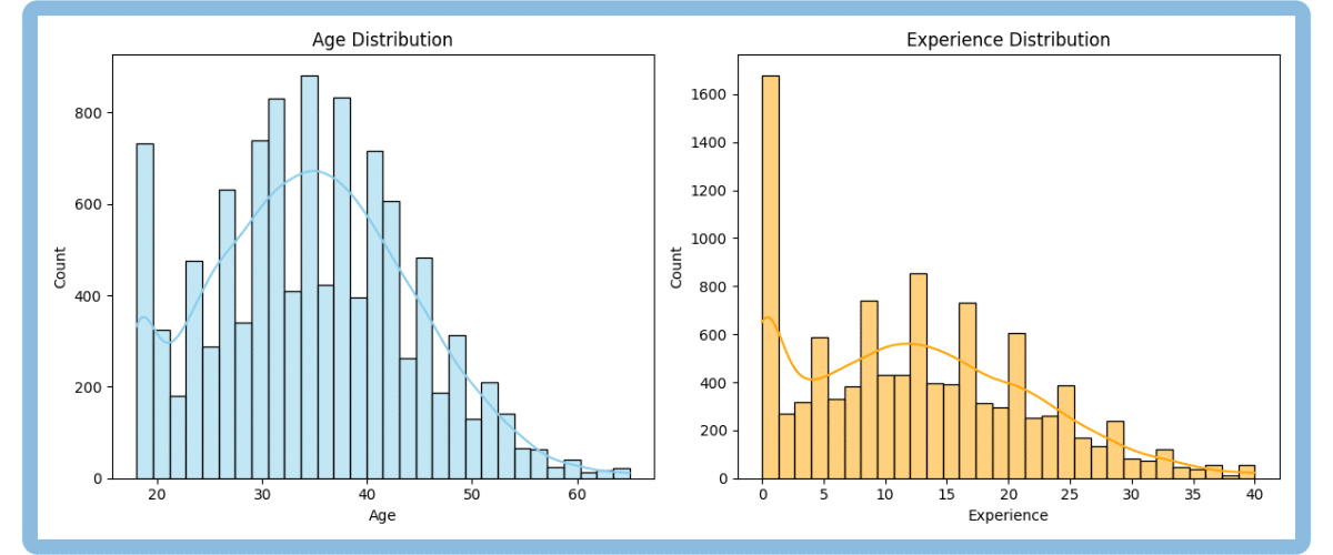
Before imputing missing values in numerical columns, we first check each column’s distribution and skewness. This matters because the best imputation strategy depends on the shape of the data:
- If the distribution is roughly symmetric (low skewness, between -0.5 and +0.5), the mean is a good choice, it fairly represents “the center” of the data.
- If the distribution is skewed (skewness outside -0.5 to +0.5), the median is better, since it isn’t affected by outliers.
# Visual check of distributions for numerical columns
fig, axes = plt.subplots(1, 2, figsize=(12, 5))
sns.histplot(employment_data['Age'].dropna(), bins=30, kde=True, color="skyblue", ax=axes[0])
axes[0].set_title('Age Distribution')
axes[0].grid(False)
sns.histplot(employment_data['Experience'].dropna(), bins=30, kde=True, color="orange", ax=axes[1])
axes[1].set_title('Experience Distribution')
axes[1].grid(False)
plt.tight_layout()
plt.show()
Output:
# Impute based on skewness
numerical_columns = ['Age', 'Experience']
for col in numerical_columns:
    skewness = employment_data[col].skew()
    print(f"{col} skewness: {skewness:.2f}")
    if abs(skewness) > 0.5:
        impute_val = employment_data[col].median()
        method = 'median'
    else:
        impute_val = employment_data[col].mean()
        method = 'mean'
    missing_count = employment_data[col].isnull().sum()
    employment_data[col] = employment_data[col].fillna(impute_val)
    print(f"{col}: Filled {missing_count} missing values with {method} ({impute_val:.2f})")
Output:
Age skewness: 0.22
Age: Filled 209 missing values with mean (34.68)
Experience skewness: 0.45
Experience: Filled 313 missing values with mean (12.58)
The skewness for both columns is less than 0.5, so the data is approximately symmetric. That’s why we use the mean for imputation. It is as simple as that.
4. Handle Categorical Missing Values:
# Handle categorical missing values
categorical_columns = ['Gender', 'Department', 'Hired', 'Location']
for col in categorical_columns:
    missing_count = employment_data[col].isnull().sum()
    employment_data[col] = employment_data[col].fillna('Unknown')
    print(f"{col}: Filled {missing_count} missing values with 'Unknown'")
Output:
Gender: Filled 2126 missing values with 'Unknown'
Department: Filled 2243 missing values with 'Unknown'
Hired: Filled 2171 missing values with 'Unknown'
Location: Filled 2214 missing values with 'Unknown'
5. Handle Date Missing Values:
# Leave date missing values as NaT
missing_dates = employment_data['Hiring_Date'].isnull().sum()
print(f"Hiring_Date: {missing_dates} missing values remain (left as NaT to preserve analytical integrity).")
Output:
Hiring_Date: 1126 missing values remain (left as NaT to preserve analytical integrity)- Missing date values were left as NaT to avoid inserting false information and to preserve the integrity of time-based analyses. Alternatives like placeholder dates, deletion, or imputation risk introducing bias or data loss, so they should be used cautiously and only if analytically justified.
6. Standardize Gender values:
# Standardize Gender values
print("Standardizing Gender values...")
print("Before:", employment_data['Gender'].value_counts())
gender_mapping = {'M': 'Male', 'F': 'Female', 'Male': 'Male', 'Female': 'Female', 'Unknown': 'Unknown'}
employment_data['Gender'] = employment_data['Gender'].map(gender_mapping)
print("After:", employment_data['Gender'].value_counts())
Output:
Standardizing Gender values...
Before: Gender
Female     2684
Male       2588
Unknown    2126
F          1849
M          1743
Name: count, dtype: int64
After: Gender
Female     4533
Male       4331
Unknown    2126
Name: count, dtype: int64
7. Standardize Hired Status:
# Standardize Hired status
print("Standardizing Hired status...")
print("Before:", employment_data['Hired'].value_counts())
hired_mapping = {'Y': 'Yes', 'N': 'No', 'Yes': 'Yes', 'No': 'No', 'Unknown': 'Unknown'}
employment_data['Hired'] = employment_data['Hired'].map(hired_mapping)
print("After:", employment_data['Hired'].value_counts())
Output:
Standardizing Hired status...
Before: Hired
Yes        3514
Y          2589
Unknown    2171
No         1774
N           942
Name: count, dtype: int64
After: Hired
Yes        6103
No         2716
Unknown    2171
Name: count, dtype: int64
8. Duplicates removal:
print(f"Dataset shape before: {employment_data.shape}")
employment_data_clean = employment_data.drop_duplicates()
print(f"Dataset shape after: {employment_data_clean.shape}")
print(f"Duplicates removed: {len(employment_data) - len(employment_data_clean)}")
Output:
Dataset shape before: (10990, 9)
Dataset shape after: (10500, 9)
Duplicates removed: 490
9. Outliers Detection:
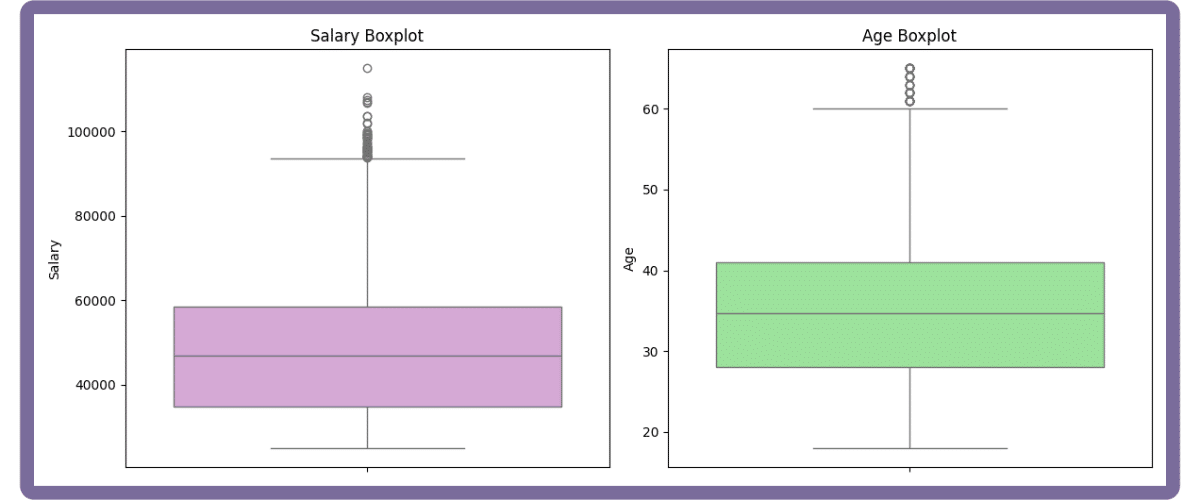
Outlier detection ensures analytical reliability by identifying values that deviate significantly from the rest. Use a boxplot for a quick visual check, then apply the IQR rule:
- A value is an outlier if it’s below (Q1 – 1.5*IQR) or above (Q3 + 1.5*IQR).
This distribution-agnostic method effectively catches most anomalies.
# Combined boxplots for key numerical columns (in subplots) and outlier reporting
fig, axes = plt.subplots(1, 2, figsize=(12, 5))
sns.boxplot(y=employment_data_clean['Salary'], ax=axes[0], color="plum")
axes[0].set_title('Salary Boxplot')
axes[0].set_ylabel('Salary')
axes[0].grid(False)
sns.boxplot(y=employment_data_clean['Age'], ax=axes[1], color="lightgreen")
axes[1].set_title('Age Boxplot')
axes[1].set_ylabel('Age')
axes[1].grid(False)
plt.tight_layout()
plt.show()
Output:
for col in ['Salary', 'Age']:
    col_data = employment_data_clean[col].dropna()
    Q1 = col_data.quantile(0.25)
    Q3 = col_data.quantile(0.75)
    IQR = Q3 - Q1
    lower = Q1 - 1.5 * IQR
    upper = Q3 + 1.5 * IQR
    outliers = ((col_data < lower) | (col_data > upper)).sum()
    print(f"{col}: {outliers} outliers detected using IQR method.")
Output:
Salary: 48 outliers detected using IQR method.
Age: 50 outliers detected using IQR method.
How you handle outliers depends on their origin:
- Correct or remove them if they’re data entry errors.
- If they are genuine but rare events, it’s often better to keep them.
- When removal isn’t possible, use robust statistics like the median or analyze the data with and without the outliers to gauge their impact.
- Always document your outlier handling for transparency and reproducibility.
10. Save the Cleaned Dataset:
# Save cleaned dataset
employment_data_clean.to_csv('employment_dataset_clean.csv', index=False)
print("✓ Cleaned dataset saved successfully!")
Output:
✓ Cleaned dataset saved successfully!Automating the Cleaning Process
1. Creating a reusable function:
def comprehensive_data_cleaning(df):
    """Comprehensive data cleaning function with visualization and IQR outlier reporting."""
    import matplotlib.pyplot as plt
    import seaborn as sns

    print("Starting automated cleaning...")
    df_clean = df.copy()

    # Data type corrections
    if 'Experience' in df_clean.columns:
        df_clean['Experience'] = df_clean['Experience'].astype(str).str.extract(r'(\d+)').astype(float)
    if 'Hiring_Date' in df_clean.columns:
        df_clean['Hiring_Date'] = pd.to_datetime(df_clean['Hiring_Date'], errors='coerce')

    # Impute after inspecting distribution/skew
    for col in ['Age', 'Experience']:
        if col in df_clean.columns:
            skewness = df_clean[col].skew()
            if abs(skewness) > 0.5:
                impute_val = df_clean[col].median()
            else:
                impute_val = df_clean[col].mean()
            df_clean[col] = df_clean[col].fillna(impute_val)

    # Handle categorical missing values
    categorical_cols = df_clean.select_dtypes(include=['object']).columns
    for col in categorical_cols:
        if col != 'Hiring_Date':
            df_clean[col] = df_clean[col].fillna('Unknown')

    # Leave date missing values as NaT

    # Standardize categorical values
    if 'Gender' in df_clean.columns:
        gender_mapping = {'M': 'Male', 'F': 'Female', 'Male': 'Male', 'Female': 'Female'}
        df_clean['Gender'] = df_clean['Gender'].map(gender_mapping).fillna(df_clean['Gender'])
    if 'Hired' in df_clean.columns:
        hired_mapping = {'Y': 'Yes', 'N': 'No', 'Yes': 'Yes', 'No': 'No'}
        df_clean['Hired'] = df_clean['Hired'].map(hired_mapping).fillna(df_clean['Hired'])

    # Remove duplicates
    initial_rows = len(df_clean)
    df_clean = df_clean.drop_duplicates()
    duplicates_removed = initial_rows - len(df_clean)
    print(f"Removed {duplicates_removed} duplicate rows")

    # Outlier detection (report only)
    for col in ['Salary', 'Age']:
        if col in df_clean.columns:
            col_data = df_clean[col].dropna()
            Q1 = col_data.quantile(0.25)
            Q3 = col_data.quantile(0.75)
            IQR = Q3 - Q1
            lower = Q1 - 1.5 * IQR
            upper = Q3 + 1.5 * IQR
            outliers = ((col_data < lower) | (col_data > upper)).sum()
            print(f"{col}: {outliers} outliers detected using IQR method.")

    return df_clean
2. Testing the Automated Cleaning Function:
# Test automated function
original_data = pd.read_csv('../input/employment-dataset-csv-data-cleaning-practice-set/employment_dataset.csv')
auto_cleaned_data = comprehensive_data_cleaning(original_data)
print(f"Original shape: {original_data.shape}")
print(f"Cleaned shape: {auto_cleaned_data.shape}")
print(f"Missing values remaining: {auto_cleaned_data.isnull().sum().sum()}")

print("=== FINAL VALIDATION ===")
print(f"✓ Dataset shape: {employment_data_clean.shape}")
print(f"✓ Missing values: {employment_data_clean.isnull().sum().sum()}")
print(f"✓ Duplicates: {employment_data_clean.duplicated().sum()}")
print(f"✓ Gender values: {sorted(employment_data_clean['Gender'].unique())}")
print(f"✓ Hired values: {sorted(employment_data_clean['Hired'].unique())}")
Output:
Starting automated cleaning...
Removed 490 duplicate rows
Salary: 48 outliers detected using IQR method.
Age: 50 outliers detected using IQR method.
Original shape: (10990, 9)
Cleaned shape: (10500, 9)
Missing values remaining: 1081
=== FINAL VALIDATION ===
✓ Dataset shape: (10500, 9)
✓ Missing values: 1081
✓ Duplicates: 0
✓ Gender values: ['Female', 'Male', 'Unknown']
✓ Hired values: ['No', 'Unknown', 'Yes']
This cleaning process refined the dataset to 10,500 analysis-ready records, with missing values handled, formats standardized, data types corrected, and outliers identified for further analytical decisions.
Building Your Data Cleaning Expertise
Data cleaning is more than a technical skill:
- it’s a mindset focused on quality and reliability.
- It’s an iterative process where experience builds intuition.
- The goal isn’t to achieve absolute perfection but to create a dataset that is reliable enough to support confident, data-driven decisions.
Take Your Data Skills to the Next Level
Ready to deepen your expertise? Udacity offers several programs to accelerate your learning journey.
The Data Analyst Nanodegree provides comprehensive training in cleaning, analysis, and visualization with Python and SQL. For those looking to advance, the Machine Learning Engineer Nanodegree builds on data preparation skills to cover model development and deployment. To focus on solving business problems, the Business Analytics Nanodegree emphasizes translating clean data into actionable insights.