Jupyter Notebook Tutorial: A Beginner’s Guide for the Data Science Tool

Introduction

In the vast landscape of data science, where exploration, analysis, and communication are paramount, one tool stands out as an indispensable companion: Jupyter Notebook. More than just a code editor, Jupyter provides an interactive computing environment that weaves together live code, equations, visualizations, and narrative text into a single, shareable document.

This unique blend makes Jupyter Notebook the go-to platform for data scientists to explore datasets, prototype models, visualize findings, and present their work in a compelling, step-by-step manner.

If you’re looking to enhance your data science workflow, this tutorial is your ultimate guide to mastering Jupyter Notebook, from setup to best practices. I still remember my true introduction to Jupyter Notebook, back around 2019. It was during an exercise for the Boston House Price Prediction model in my Data Scientist Nanodegree program. Before that, my workflow for any data analysis involved writing long, monolithic .py scripts, running them from the command line, and then tediously taking screenshots of pop-up plots and console outputs to piece together reports. It was a fragmented and inefficient process.

Discovering Jupyter Notebook, with its interactive cells where I could run code, see immediate results, and embed visualizations and explanatory text all in one place, was a complete game-changer. It transformed how I explored data and built models, making the entire analytical journey intuitive and truly collaborative.

At its core, a Jupyter Notebook is an open-source web application that allows you to create and share documents containing live code, equations, visualizations, and explanatory text. The “Jupyter” name itself is a reference to the three core programming languages supported by the Jupyter Project: Julia, Python, and R. While it supports many languages through its “kernels,” Python remains the most widely used.

Its importance in data science stems from several key aspects:

• Interactivity: Execute code cell by cell, allowing for immediate feedback and iterative development.
• Literate Programming: Combine code with rich text (Markdown), images, and equations to explain your thought process directly alongside your analysis.
• Reproducibility: Capture your entire analytical workflow, making it easier for others (or your future self) to understand and reproduce your results.
• Exploration & Visualization: Seamlessly integrate powerful data visualization libraries to generate plots and charts directly within the notebook output.
• Collaboration & Sharing: Easily share your work in a self-contained, human-readable format.

Setting up Jupyter Notebook

Getting Jupyter Notebook installed and ready to use is quite straightforward. There are two primary recommended methods:

1. Via Anaconda (Recommended for Beginners):

Anaconda is a popular open-source distribution for Python and R that simplifies package management and deployment. It comes bundled with Jupyter Notebook and many other essential data science libraries (like NumPy, Pandas, Matplotlib, and Scikit-learn).

• Download:
  Visit the official Anaconda website at: https://www.anaconda.com/products/distribution and download the appropriate installer for your operating system (Windows, macOS, Linux).
• Install:
  Follow the installation wizard’s instructions. It’s generally recommended to use the default settings.
• Launch:
  Once installed, open the “Anaconda Navigator” application, and you’ll see a launch button for Jupyter Notebook. Alternatively, open your terminal or command prompt and type:

jupyter notebook

2. Via pip (for Existing Python Environments):

If you already have Python installed and prefer to manage packages with pip (and ideally use a virtual environment), you can install Jupyter Notebook directly.

• Create/Activate Virtual Environment (Recommended):

python —m venv myenv 
source myenv/bin/activate # On Windows: myenv\Scripts\activate

• Install Jupyter:

pip install notebook

• Launch:

jupyter notebook

After running the launch command, Jupyter will start a local server and open a new tab in your default web browser (usually at http://localhost:8888).

Navigating the Interface

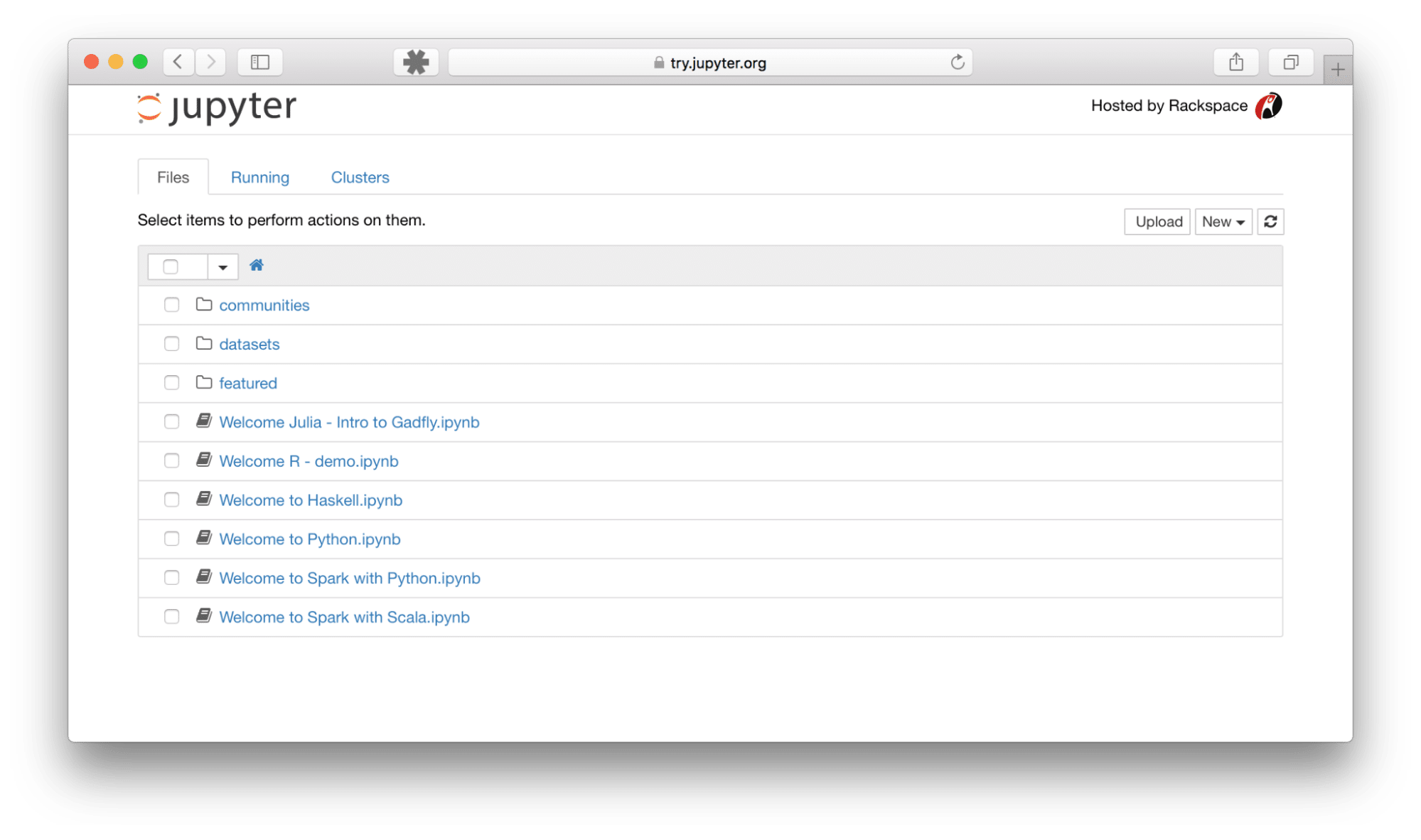
When you launch Jupyter Notebook, you’ll first see the Dashboard in your web browser, which acts as a file browser and session manager. Here, you can navigate your file system, create new notebooks, open existing ones, and manage running processes.

When you open or create a new notebook, you enter the Notebook Interface, which is where the magic happens. Key components include:

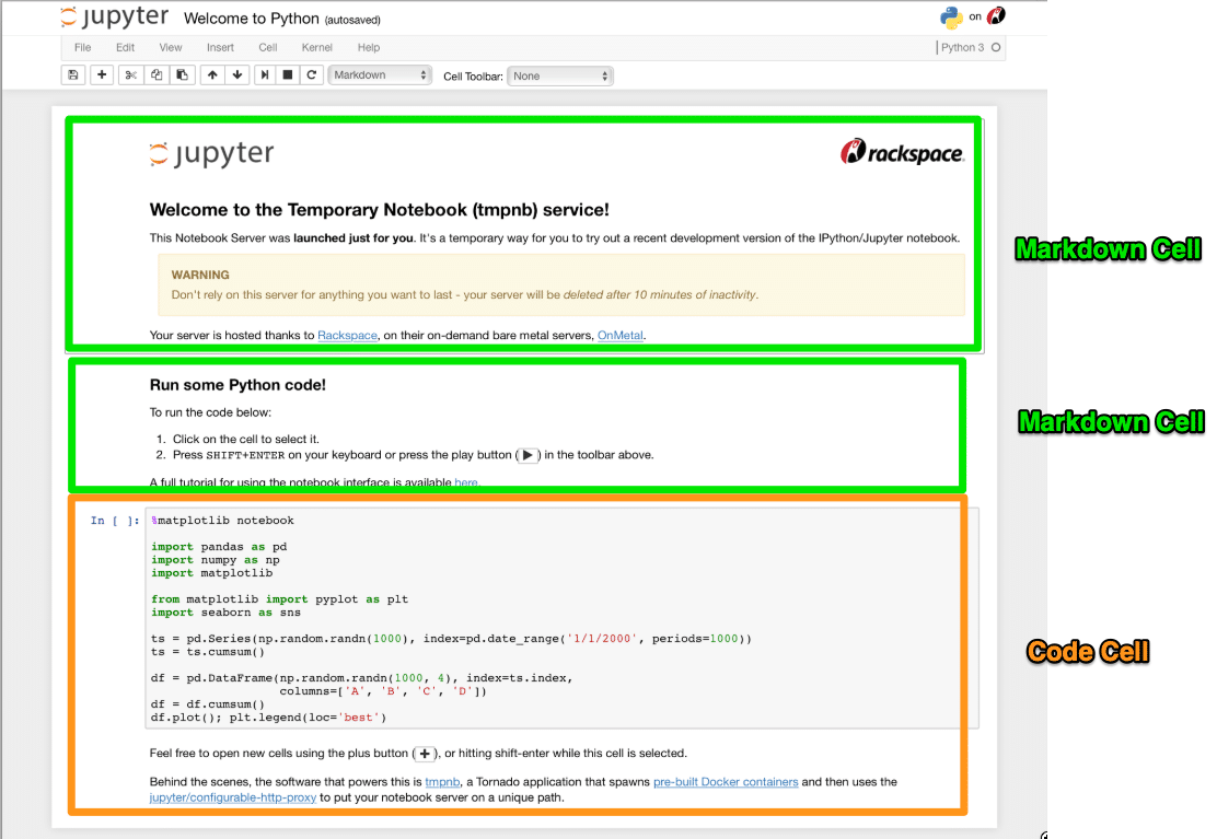
1. Cells:

The fundamental building blocks. A notebook is composed of a sequence of cells.

• Code Cells: Where you write and execute code. The output appears directly below the cell.
• Markdown Cells: Where you write explanatory text using Markdown syntax, which can include headings, bold text, lists, links, images, and even LaTeX equations.

2. Kernel:

This is the “computational engine” that runs the code in your notebook. When you execute a code cell, the code is sent to the kernel, processed, and the results are sent back to the notebook. You can restart, interrupt, or change the kernel via the “Kernel” menu.

3. Menu Bar:

At the top, providing standard options like File (New Notebook, Open, Save, Download As), Edit (Cut, Copy, Paste cells), View, Insert (Insert Cell Above/Below), Cell (Run All, Run Selected), Kernel (Restart, Interrupt), Widgets, and Help.

4. Toolbar:

A set of quick-access icons below the Menu Bar for common actions: Save, Insert Cell, Cut/Copy/Paste Cell, Move Cell Up/Down, Run Cell, Interrupt Kernel, Restart Kernel, and Cell Type dropdown (Code/Markdown/Raw NBConvert).

Writing and Executing Code

The core of using Jupyter Notebooks for data science lies in its code cells.

1. Select a Code Cell:

 Click on an empty code cell or insert a new one (using the + button in the toolbar or Insert > Cell Below).

2. Type your Code:

Write your Python code directly into the cell.

# This is a code cell example
name = "Jupyter"
version = 5

print(f"Hello from {name} Notebook! Version {version}.")

x = 10
y = 25
z = x * y
print(f"The product of {x} and {y} is {z}")

3. Execute the Code:

• Press Shift + Enter: Runs the current cell and selects the next cell below it (or inserts a new one if you’re at the bottom).
• Press Ctrl + Enter: Runs the current cell and keeps the current cell selected.
• Click the “Run” button (►) in the toolbar.

The output of your code (e.g., print statements, variable values if they are the last line of the cell) will appear directly below the code cell. You can also use Magic Commands, special commands prefixed with % (line magic) or %% (cell magic), for useful functionalities like timing code (%%time) or integrating plots (%matplotlib inline).

Data Visualization

Jupyter Notebooks truly shine when it comes to data visualization, allowing you to generate and display plots directly within your workflow. This interactivity is crucial for exploratory data analysis.

First, you’ll typically use a “magic command” to ensure plots are rendered inline within the notebook:

%matplotlib inline

Now, let’s integrate popular Python visualization libraries:

1. Matplotlib:

A foundational plotting library.

import matplotlib.pyplot as plt
import numpy as np
# Generate some sample data
x = np.linspace(0, 10, 100)
y = np.sin(x)
# Create a simple line plot
plt.plot(x, y)
plt.title("Sine Wave")
plt.xlabel("X-axis")
plt.ylabel("Y-axis")
plt.grid(True)
plt.show()

2. Seaborn:

Built on Matplotlib, providing a high-level interface for drawing attractive statistical graphics.

import seaborn as sns
import pandas as pd

# Create a simple DataFrame
data = {'Category': ['A', 'B', 'C', 'D', 'E'],
        'Value': [23, 45, 56, 12, 39]}
df = pd.DataFrame(data)

# Create a bar plot
sns.barplot(x='Category', y='Value', data=df)
plt.title("Category Values")
plt.show()

The resulting plots will magically appear directly below the code cells that generated them, making your analysis immediately visual and understandable.

Sharing and Exporting Notebooks

Jupyter Notebooks are fantastic for sharing your work. The native file format is .ipynb, which is a JSON file containing all your code, output, and Markdown.

1. Direct Sharing:

 You can share the .ipynb file directly with collaborators. They can open it in their own Jupyter environment.

2. GitHub:

GitHub has native rendering for .ipynb files. If you push a notebook to a GitHub repository, it will be displayed directly in the browser, making it a great way to showcase projects.

3. Google Colaboratory (Colab):

A cloud-based Jupyter environment from Google that allows you to run notebooks entirely in the browser, often with free GPU access. You can upload and share notebooks directly from/to Colab.

4. nbviewer:

A free web service that renders any public Jupyter Notebook directly from a URL (e.g., from a GitHub Gist or repository). Paste the link to your .ipynb file there, and it will render beautifully.

5. Exporting to Various Formats:

Jupyter Notebook allows you to export your work into several static formats via File > Download as:

• .ipynb (Notebook): The native format.
• .py (Python Script): Extracts only the code cells into a standard Python script.
• .html (HTML): Creates a static web page version of your notebook, complete with code and outputs. Great for sharing with non-technical audiences.
• .pdf (PDF): Requires Pandoc and a LaTeX distribution (like MiKTeX for Windows or MacTeX for macOS) to be installed on your system.
• .md (Markdown): Converts all content to Markdown format.

You can also use the Jupyter nbconvert command-line tool for more advanced conversions:

# Convert to HTML
jupyter nbconvert --to html your_notebook.ipynb

# Convert to Python script
jupyter nbconvert --to script your_notebook.ipynb

Best Practices for Effective Notebook Usage

To truly leverage Jupyter Notebooks and avoid common pitfalls, adopt these best practices:

• Use Markdown Extensively: Don’t just write code! Use Markdown cells to explain your thought process, describe data sources, outline steps, interpret results, and add context. A well-documented notebook is a joy to read.
• Keep Cells Concise and Focused: Break down complex logic into smaller, manageable code cells. Each cell should ideally perform a single, logical step. This improves readability and debugging.
• Run Cells in Order: Always execute cells sequentially from top to bottom. Jupyter maintains the state of your kernel, and skipping cells or running them out of order can lead to unexpected errors.
• Restart Kernel Frequently: Especially during active development, restart your kernel (Kernel > Restart) to clear all variables and ensure your code runs cleanly from scratch. This helps catch dependencies on previously run, but now removed, code.
• Clear Outputs Before Sharing/Committing: For smaller file sizes and to protect sensitive outputs, clear all outputs (Cell > All Output > Clear) before saving and sharing or committing to version control.
• Leverage Version Control (Git): Use Git to track changes to your notebooks. While .ipynb files can be challenging for Git diffs, services like GitHub render them, making it valuable for project history.
• Utilize Virtual Environments: Always work within a dedicated virtual environment for each project to manage dependencies and avoid conflicts between different projects.
• Use Comments in Code: Even with Markdown explanations, internal code comments remain crucial for complex logic within a cell.

Continue your Journey

Jupyter Notebook is more than just a tool; it’s an ecosystem that fundamentally transforms the way data science projects are conducted. Its interactive nature, ability to weave code and narrative, and seamless integration with powerful libraries make it an indispensable asset for exploration, analysis, visualization, prototyping and communication.

By following this tutorial, you’ve taken the first significant step towards mastering this incredible environment. To truly transform your understanding of data and master the full spectrum of a data analyst’s mental model, consider Udacity’s Data Analyst Nanodegree program. This comprehensive program builds directly on the foundational skills you’ve gained with Jupyter Notebooks, equipping you to handle real-world data challenges.

You’ll dive deep into:

• Introduction to Data Analysis with Pandas and NumPy: Mastering core data manipulation and basic visualizations, refining your exploratory data analysis techniques, and understanding the complete data analysis process – all within the interactive environment of Jupyter.
• Advanced Data Wrangling: Developing crucial skills in data cleaning, assessing data tidiness and quality, effective data gathering, and efficient file I/O for robust data preparation.
• Data Visualization with Matplotlib and Seaborn: Elevating your visualization capabilities by mastering design principles, understanding data limitations and biases, and crafting professional presentations that tell compelling data stories.

This Nanodegree will empower you to not only use tools like Jupyter but to confidently navigate complex datasets, derive meaningful insights, and communicate them effectively, preparing you for a successful career in data analytics.