Data Modeling 101: How to Structure Your Data for Maximum Insight

Data modeling is a cornerstone of effective data analytics and engineering. Without a well-structured data model, even the most advanced tools and algorithms can fall short of delivering actionable insights. This guide will walk you through the essentials of data modeling, from understanding its importance to applying best practices for building reliable and efficient data systems.

Introduction

Data modeling turns questions into structures that software can rely on. If someone asks “Which products drive repeat purchases?” or “How much did we sell last week?”, clear tables and relationships let you answer quickly and confidently. Without a model, simple questions often become slow, error-prone, and expensive.

Our hypothetical T-shirt shop wants to know daily revenue, best-selling products, and which customers come back. We will start with a conceptual picture, refine it into a logical model with keys and attributes, then implement a small physical schema. Finally, we will show how to reshape the same data for analytics with a compact star schema.

Types of Data Models

1) Conceptual data model

This is the map of business ideas, not columns.

• Customer places Order.
• Order contains OrderItems for Product.

Concepts and relationships:

1. Entities: Customer, Order, OrderItem, Product.

2. Relationships:

• Customer 1..* Order.
• Order 1..* OrderItem.
• Product 1..* OrderItem.

2) Logical data model

Now, we attach attributes and keys, while staying independent of any database engine.

• Customer(customer_id PK, email, created_at, country)
• Product(product_id PK, sku, name, color, size, list_price, category)
• Order(order_id PK, customer_id FK, order_ts, status, currency, total_paid, refunded_amount optional)
• OrderItem(order_item_id PK, order_id FK, product_id FK, qty, unit_price, discount_amount, tax_rate)

Design choices for the simplified scenario:

• unit_price lives on OrderItem so historical orders do not change when list_price changes in Product.
• refunded_amount is an optional column on Order so we can demonstrate net revenue without introducing a separate refunds table.

3) Physical data model

Here is a compact PostgreSQL implementation that mirrors the logical model.

CREATE TABLE customers (
  customer_id VARCHAR PRIMARY KEY,
  email TEXT NOT NULL UNIQUE,
  created_at TIMESTAMPTZ NOT NULL DEFAULT NOW(),
  country TEXT
);

CREATE TABLE products (
  product_id VARCHAR PRIMARY KEY,
  sku TEXT NOT NULL UNIQUE,
  name TEXT NOT NULL,
  color TEXT,
  size TEXT,
  list_price NUMERIC(10,2) NOT NULL,
  category TEXT
);

CREATE TABLE orders (
  order_id VARCHAR PRIMARY KEY,
  customer_id BIGINT NOT NULL REFERENCES customers(customer_id),
  order_ts TIMESTAMPTZ NOT NULL,
  status TEXT NOT NULL,
  currency TEXT NOT NULL,
  total_paid NUMERIC(10,2) NOT NULL DEFAULT 0,
  refunded_amount NUMERIC(10,2) NOT NULL DEFAULT 0,
  CHECK (total_paid >= 0),
  CHECK (refunded_amount >= 0)
);

CREATE INDEX ON orders (customer_id, order_ts);

CREATE TABLE order_items (
  order_item_id VARCHAR PRIMARY KEY,
  order_id BIGINT NOT NULL REFERENCES orders(order_id),
  product_id BIGINT NOT NULL REFERENCES products(product_id),
  qty INT NOT NULL CHECK (qty > 0),
  unit_price NUMERIC(10,2) NOT NULL,
  discount_amount NUMERIC(10,2) NOT NULL DEFAULT 0,
  tax_rate NUMERIC(5,4) NOT NULL DEFAULT 0
);

That is the complete operational model, including: Four tables, a few constraints, and one helpful index for frequent “recent orders by customer” queries.

Note: Production systems often add more constraints, indexes, and history tracking. For instance, changes to product details should be recorded, and ideally include the information on who made the edits and when. As another example, it is generally a good practice to have created_at and updated_at columns in all tables.

Key Data Modeling Concepts

A strong understanding of fundamental concepts is essential for successful data modeling:

• Entities represent things we store. Here they are Customer, Product, Order, and OrderItem.
• Relationships define how those things connect. One Customer can place many Orders. Each Order has many OrderItems. Each OrderItem points to one Product.
• Primary keys uniquely identify rows. We use surrogate keys (BIGSERIAL) so joins stay stable even if business identifiers change.
• Foreign keys enforce integrity. order_items.product_id must exist in products.product_id. This prevents orphan lines.
• Cardinality captures real rules. An Order has one or more OrderItems. An OrderItem references exactly one Product.

Suppose a customer buys 2 “Classic Tee, blue, M” at 15.00 each and 1 “Logo Tee, black, L” at 18.00. We record:

1. One row in orders with total_paid = 48.00.
2. Two rows in order_items:

• qty = 2, unit_price = 15.00, discount_amount = 0
• qty = 1, unit_price = 18.00, discount_amount = 0

If a partial refund of 15.00 occurs, set refunded_amount on the related order to 15.00. Note that keeping refunds as a single field on the orders table is not necessarily a good practice because it collapses multiple financial events into one value, hides line-level context, and weakens auditability; in a real-world scenario you would store refunds in a separate refunds table so that each refund is captured as its own record with amount, timestamp, method, reason, status, and an optional link to the specific order_item, enabling multiple partial refunds, per-line refunds, accurate reconciliation, and clear constraints.

Common Modeling Techniques

Several tried-and-true techniques help translate ideas into robust data structures:

1. Entity-Relationship (ER) Diagrams:

Visual representations of entities and their relationships. These diagrams make it easier to communicate the structure of the data to both technical and non-technical stakeholders.

2. Normalization:

Normalization structures tables to reduce redundancy and prevent anomalies during insert, update, and delete operations. The goal is a schema where each fact is stored in one place and remains consistent over time.

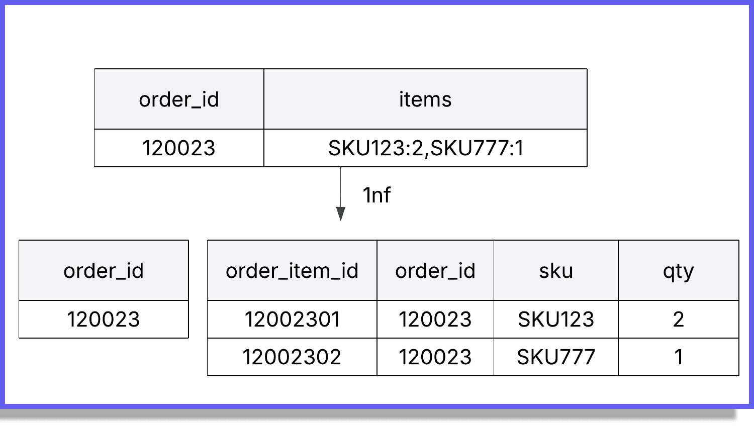
First Normal Form (1NF)

A table is in 1NF when:

• Each row is uniquely identified by a primary key.
• Each column holds atomic values only, with no arrays or repeating groups.
• Each column has a single, consistent meaning and data type.

Quick check: every cell contains one value, not a list or JSON blob, for example:

• Violation: A column like orders.items storing “SKU123:2,SKU777:1” or a JSON array of lines.
• Fix: Move items into order_items with one row per product per order. Each cell holds a single value.

Second Normal Form (2NF)

A table is in 2NF when:

• It is already in 1NF.
• Every non key column depends on the whole primary key, not just part of it.

2NF matters when a table uses a composite primary key. If a non key attribute depends on only one part of that composite key, move it to a table keyed by that part. For example:

Assume order_items uses a composite key (order_id, product_id).

Violations:

• Storing order_ts in order_items. It depends only on order_id.
• Storing product_name in order_items. It depends only on product_id.

Fix:

• Keep order_ts in orders, and product_name in products. Keep in order_items only attributes that depend on both order_id and product_id, such as qty, unit_price, and discount_amount.

Third Normal Form (3NF)

A table is in 3NF when:

• It is already in 2NF.
• There are no transitive dependencies. Every non key column depends on the key, the whole key, and nothing but the key.

Plain meaning:

No non key column should determine another non key column. If A determines B and neither is a key, B belongs in a table where A is the key.

Why 3NF matters?

Removing transitive dependencies eliminates hidden duplication and conflicting updates, keeps each fact authoritative in one location, and simplifies constraints and queries.

As an example, in the orders table:

Violation:

• Keeping customer_email in orders alongside customer_id. Since customer_id -> customer_email, this is a transitive dependency.

Fix:

• Store customer_email only in customers and reference it via customer_id when needed.

Beyond 3NF

Higher forms such as Boyce Codd Normal Form (BCNF), 4NF, and 5NF exist, but they address specialized dependency patterns and are not commonly required in most lines of business systems. For operational databases, 3NF is a practical target. For analytics, star schemas intentionally denormalize to make queries simpler and faster.

As a quick note related to BCNF, it is sometimes not that rare, especially when there are overlapping candidate keys. For 4NF (multi-valued dependencies), it can be relevant in product-attribute systems (e.g., a product can have multiple colors and multiple sizes, independent attributes).

3. Star and Snowflake Schemas:

Common in data warehousing, these schemas structure data for analytical queries. A star schema has a central fact table connected to dimension tables, while a snowflake schema further normalizes dimension tables.

Building the star schema in practice

For our hypothetical T-shirt store, the analytical model favors short joins and clear grains. The normalized schema has four operational tables: customers, products, orders, and order_items. The star schema below creates two fact tables and a small set of dimensions that answer common questions such as “Net revenue by day and category” and “Units sold by size and color.”

Facts:

• fact_orders (one row per order)
• fact_order_items (one row per order item)

Dimensions:

• dim_date (calendar attributes)
• dim_products (sku, name, color, size, category)
• dim_customers (country and simple customer attributes)
• Optional: dim_currency if multiple currencies are present

Extract attributes from the normalized tables into compact dimensions with surrogate keys, then load fact tables at a declared grain. Populate dim_products from products and dim_customers from customers, generate dim_date for the full calendar range you will report on, and map each order and item to the correct dimension keys based on order timestamps and natural keys. Compute measures such as gross amount, discounts, tax, item count, and net amount during fact loads, and carry degenerate identifiers like order_id to enable drill through.

Why a dim_date table exists?

SQL engines already have a date type, but reporting usually needs richer calendar context that is awkward to compute on the fly.

A dim_date table provides one row per calendar day with attributes like date_key (YYYYMMDD), date_value, year, quarter, month, day, weekday, is_weekend, and optional fiscal fields or holiday flags.

This table is created once for a broad date range and then reused by all facts, which gives consistent time groupings, simplifies filters, and improves performance in BI tools. It also centralizes special calendars, such as a retail 4-5-4 schedule or region specific holidays, so every report uses the same definitions.

Tools for Data Modeling

The right tools can make the modeling process more efficient and collaborative. Some popular choices include:

• dbdiagram.io: An online tool for quickly sketching and sharing database diagrams.
• ER/Studio: A professional modeling solution with advanced collaboration features.
• Lucidchart: A versatile diagramming tool that supports ER diagrams along with many other diagram types.

These tools help teams visualize, refine, and maintain their data models, often providing export options for direct database implementation.

Best Practices

To create effective data models, consider these best practices:

• Avoid Redundancy: Duplicate data increases storage needs and risk of inconsistency. Normalization and proper relationships can help.
• Ensure Data Integrity: Use constraints, primary/foreign keys, and validation rules to maintain accuracy and consistency.
• Model for the Future: Anticipate changes in business needs and design with scalability in mind.
• Involve Stakeholders: Collaborate with business users, analysts, and engineers to ensure the model reflects real-world requirements.

Conclusion

Data modeling is more than just a technical step. It’s the foundation of a successful analytics and engineering strategy. By carefully designing your data structures, you can reduce errors, improve performance, and make your data more accessible and meaningful.

Before jumping into building and maintaining models, take the time to model your data thoughtfully. Doing so will save countless hours of troubleshooting later and ensure your analytics deliver the insights you need.If you want structured practice that takes you from modeling and SQL to pipelines and warehouses, explore Udacity’s courses in the School of Data Science, in particular, Programming for Data Science with Python and Data Engineering with AWS. They include hands-on projects that mirror real systems and teach you how to design, build, and maintain analytics-ready data.