Last Updated on February 20, 2025
When I first started developing e-commerce applications, I was so focused on the user interface and site performance that I seldom gave thought to the math running under the hood. Over time, I realized that behind most successful tech products—especially those involving product recommendations, search rankings, and personalizations—there’s a powerful optimization algorithm known as gradient descent.
Gradient descent is central to modern machine learning and optimization. Whether you’re training a neural network, building a regression model, or fine-tuning a recommendation system, chances are you’ll rely on gradient descent to make everything run smoothly. This article provides a deep dive into gradient descent optimization, offering an overview of what it is, how it works, and why it’s essential in machine learning and AI-driven applications.
Whether you’re a data scientist, a technology professional, or simply curious about how data-driven solutions are built, gradient descent can open a whole new world of opportunities. Let’s explore it step by step.
Table of Contents
Common Challenges and How to Overcome Them
Applications of Gradient Descent
What Is Gradient Descent?
At its core, gradient descent is a first-order iterative optimization algorithm for finding the local minimum of a differentiable function. In more direct terms, imagine you have a function 𝑓(𝑥) that outputs a measure of error (often called a “cost” or “loss”). The goal is to adjust the parameters 𝑥 in such a way as to minimize this cost function.
From a geometric perspective, you can think of the cost function as a landscape—mountains, valleys, hills, and troughs. The job of gradient descent is to get you from your starting point at the top of some slope (or random location) down to the lowest valley. It does this by moving in the direction opposite to the gradient. Here’s an image generated via Python to illustrate this concept:
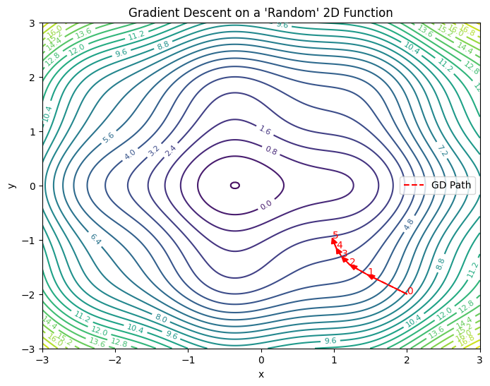
The GD Path is the path taken by the gradient descent algorithm to get to the lowest point (0.0). Notice the distances get shorter in subsequent iterations. These distances are determined by the learning rate. More on this later.
Why It’s Essential for Training Machine Learning Models
In machine learning, we often have a set of parameters (weights, biases, etc.) whose values we want to optimize to minimize the error between our model’s predictions and the ground truth. Gradient descent is the most common method for doing so because:
- Computational Efficiency: It’s relatively straightforward to calculate gradients, even for large datasets and complex models.
- Scalability: Gradient-based optimizations scale well, making them suitable for massive neural networks and huge datasets.
- Generality: You can apply gradient descent to a wide variety of models—linear, logistic, deep neural networks, and more.
How Gradient Descent Works
To understand the mechanics of gradient descent, let’s outline the step-by-step procedure:
- Initialize Parameters
Start by initializing your model parameters (e.g., weights and biases in a neural network) to some random values or a specific distribution. For a simple example, let’s denote our single parameter as x. - Compute the Cost Function
Calculate the cost (or loss) based on your current parameter values. A commonly used cost function in simple regression problems is the Mean Squared Error (MSE). More generally, you might have a function f(x) that outputs how “wrong” your model is. - Compute the Gradients
The gradient is the partial derivative of the cost function with respect to the parameters. Symbolically, if f(x) is our cost function, we find dfdx. This tells us the direction in which f(x) increases the fastest. - Update the Parameters
Adjust the parameters in the direction opposite to the gradient:
x ← x−α⋅dfdx
Here, α (alpha) is called the learning rate—it controls how big a step you take on each update.
- Iterate Until Convergence
Keep repeating the previous steps—recalculate the cost, find the gradients, update parameters—until changes become negligible or you reach a preset iteration count.
Key Terms
- Cost Function (Loss Function): This tells you how far off your model’s predictions are from the actual values.
- Gradients: Partial derivatives of the cost function with respect to the parameters. They guide parameter updates.
- Learning Rate: A hyperparameter that determines the size of each update step. This is shown by the distances traveled in each step in the image above. Too large and you might overshoot; too small and training becomes painfully slow.
Types of Gradient Descent
There are three primary types of gradient descent, each differing in how they use the training data to compute the gradient.
Batch Gradient Descent
Uses the entire training dataset to compute the gradient and update parameters once per iteration (epoch). Stable and accurate, but potentially slow for massive datasets, as you need to process all training examples before a single parameter update.
Stochastic Gradient Descent (SGD)
In the strict sense, this method updates parameters using one training example (or a very small subset of size 1) at a time. Very fast, but gradient calculations can be very noisy, and training loss might fluctuate heavily.
Note: Pure SGD (1 sample at a time) is relatively rare in practice nowadays—often, people say “SGD” but actually mean “mini-batch gradient descent.”
Mini-Batch Gradient Descent
A hybrid approach that processes small batches of the training data (e.g., 32, 64, or 128 samples) at a time. This algorithm takes the best of a full-batch gradient descent and SGD, and it exploits matrix operations well on modern hardware (GPU/TPU). On the other hand, it requires tuning batch size for optimal performance; might still be somewhat noisy compared to full batch.
Technically, pure SGD is the extreme case of updating parameters per single sample, while mini-batch is often considered a more generalized or “batched” version of SGD. In other words, mini-batch can be viewed as a Stochastic Gradient Descent with a batch size > 1.
In short:
- Batch Gradient Descent = entire dataset per update.
- Mini-Batch Gradient Descent = small subset (e.g., 32 examples) per update.
- Pure Stochastic Gradient Descent = 1 example per update.
Variants of Gradient Descent Optimization
To address issues like slow convergence and local minima, researchers developed adaptive optimizers such as Momentum, RMSProp, and Adam. Momentum accumulates past gradients to smooth out updates and increase speed in consistent directions, RMSProp adapts the learning rate based on recent gradient magnitudes, and Adam combines both momentum and adaptive learning rates. Each method aims to improve training stability and speed, but selecting the right optimizer often depends on model complexity and data characteristics. For many tasks, Adam is a solid default, while a well-tuned SGD with Momentum can also perform remarkably well.
Common Challenges and How to Overcome Them
When I was working on this recommendation engine, we faced a peculiar problem: as we added more user interactions, the model started diverging. It turned out that the new data distribution was drastically different, making our originally tuned learning rate too large. The fix was simple yet so enlightening: we reduced the learning rate by a factor of 10 and then introduced a learning-rate scheduler that gradually lowered it further as training proceeded. Suddenly, the model converged smoothly—and user satisfaction metrics improved dramatically.
The point is, gradient descent can face issues like vanishing or exploding gradients, which often arise in deeper models. Proper weight initialization and techniques like batch normalization can help maintain stable gradients.
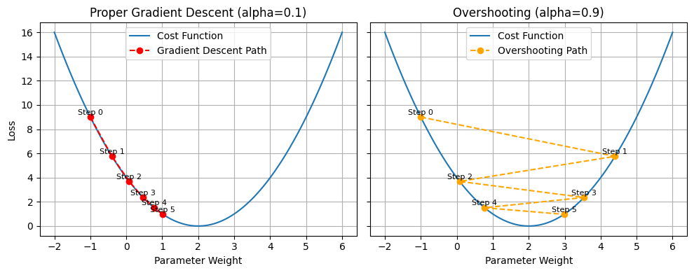
Overshooting can also occur if the learning rate is too high—using smaller rates or adaptive optimizers such as Adam typically mitigates this. As an example, an image classifier might bounce between high and low accuracy if updates overshoot.
The following graph visualizes overshooting in comparison to a proper gradient descent.
Finally, local minima or saddle points might stall progress, but momentum-based methods and varied initializations often help the model escape these pitfalls. For instance, a recommendation system could get “stuck” showing a narrow set of products until momentum-based updates push it out of a suboptimal state.
Here’s a graph illustrating the importance of the model’s initial values. Starting closer to the global minimum is a deciding factor to reaching it.

Applications of Gradient Descent
Gradient descent underpins many deep learning breakthroughs. In image classification, convolutional neural networks rely on iterative updates to refine filter weights, while in NLP, Transformers train billions of parameters via gradient-based optimizers. Recommendation engines (e.g., suggesting products in an e-commerce setting) often employ matrix factorization or deep neural networks, both of which rely on gradient descent to personalize user experiences effectively.
Python Code Example
By now you may have a vague idea of what a gradient descent algorithm is. I don’t know about you, but for me personally, I find it difficult to understand a new concept without seeing it in action.
Here’s a small Python code that sets up an example dataset, and we will use Gradient Descent to make some predictions with it. At the end of this code, there is a section to calculate the cost, a measure that tells us how similar the output of our model’s prediction compared to the correct answers. 0 means all predictions are correct.
import numpy as np

# -------------------
# 1. Generate Sample Data
# -------------------
# Let's create a small dataset of 10 points where:
#   true_slope = 2, true_intercept = 1
#   plus a bit of random noise to simulate real-world data

np.random.seed(42)  # for reproducibility
X = np.linspace(0, 5, 10)  # 10 points from 0 to 5
true_slope = 2.0
true_intercept = 1.0
noise = np.random.randn(10) * 0.5  # random noise

y = true_slope * X + true_intercept + noise

# -------------------
# 2. Define the Model and Cost Function
# -------------------
# Model: y_pred = m * x + b
# Cost Function: MSE (Mean Squared Error)

def predict(x, m, b):
    return m * x + b

def mse_loss(x, y, m, b):
    y_pred = predict(x, m, b)
    return np.mean((y_pred - y)**2)

# -------------------
# 3. Compute Gradients (via partial derivatives)
# -------------------

def compute_gradients(x, y, m, b):
    N = len(x)
    y_pred = predict(x, m, b)

    # partial derivative wrt m
    dm = (2 / N) * np.sum((y_pred - y) * x)
    # partial derivative wrt b
    db = (2 / N) * np.sum(y_pred - y)

    return dm, db

# -------------------
# 4. Gradient Descent Loop
# -------------------
# Iterate multiple times, updating m and b each iteration.

# Hyperparameters
learning_rate = 0.01
num_iterations = 100

# Initialize parameters
m = 0.0
b = 0.0

# Store cost to see how it decreases
history = []

for i in range(num_iterations):
    # Compute current cost
    cost = mse_loss(X, y, m, b)
    history.append(cost)

    # Compute gradients
    dm, db = compute_gradients(X, y, m, b)

    # Update parameters
    m -= learning_rate * dm
    b -= learning_rate * db

    # Print progress every 10 iterations
    if i % 10 == 0:
        print(f"Iteration {i}, Cost: {cost:.4f}, m: {m:.4f}, b: {b:.4f}")

# Final results
final_cost = mse_loss(X, y, m, b)
print("\nFinal Parameters:")
print(f"m = {m:.4f}, b = {b:.4f}")
print(f"Final Cost: {final_cost:.4f}")
When you run this code, you should see results like this:
Iteration 0, Cost: 48.9781, m: 0.4127, b: 0.1245
Iteration 10, Cost: 0.9228, m: 1.9484, b: 0.6086
Iteration 20, Cost: 0.2131, m: 2.1262, b: 0.6930
Iteration 30, Cost: 0.1942, m: 2.1405, b: 0.7277
Iteration 40, Cost: 0.1863, m: 2.1354, b: 0.7551
Iteration 50, Cost: 0.1793, m: 2.1283, b: 0.7805
Iteration 60, Cost: 0.1730, m: 2.1213, b: 0.8045
Iteration 70, Cost: 0.1674, m: 2.1147, b: 0.8272
Iteration 80, Cost: 0.1623, m: 2.1084, b: 0.8487
Iteration 90, Cost: 0.1578, m: 2.1024, b: 0.8691
Final Parameters:
m = 2.0973, b = 0.8865
Final Cost: 0.1537
Notice that the Cost is getting lower with each iteration. m and b are the parameters of our model, which should be close to the dataset generator’s true_slope and intercept (2 and 1, respectively).
Note: This minimal code example is intentionally written without heavy dependencies to illustrate the core gradient descent steps. In real-world applications, you’d likely use powerful libraries like PyTorch or Keras to handle everything from data loading to model training—significantly streamlining the development process.
Conclusion
Recap of Key Concepts
- Gradient Descent is a methodical approach to parameter updates, driving your model’s cost function toward a minimum.
- Types of Gradient Descent—Batch, Stochastic, and Mini-Batch—each offer trade-offs between computational cost and convergence stability.
- Adaptive Algorithms like Adam, RMSProp, and Momentum-based optimizers mitigate some of gradient descent’s inherent limitations.
- Common Challenges (vanishing/exploding gradients, overshooting, local minima) can be addressed through strategic hyperparameter tuning and advanced techniques.
- Applications in recommender systems, image classification, NLP, and even e-commerce personalization highlight the versatility of gradient descent.
Role of Gradient Descent in Optimization
In the broader context of optimization—whether you’re building a marketing campaign predictor, a product recommendation engine, or an AI-driven search system—gradient descent is at the heart of finding that “sweet spot” that maximizes user engagement and conversions.
Gradient descent can feel challenging at first, but once you understand its mechanics and practice with real-world scenarios, it becomes an invaluable tool in your developer toolbox—especially for data-driven, AI-centric applications.
If you’re intrigued and want a more structured, hands-on approach to machine learning and the optimization algorithms behind it, consider exploring Udacity’s Machine Learning Engineer Nanodegree programs. You’ll gain deeper insights into model-building, hyperparameter tuning, and how to effectively leverage gradient descent for various projects.
- Intro to Machine Learning: This is a free introduction course to get your feet wet if you are new to machine learning.
- Introduction to Machine Learning with Pytorch: If you want something more practical, you may subscribe to this course to learn how to use PyTorch to create machine learning models.
- Introduction to Machine Learning with Tensorflow: This is the Tensorflow version of the above course.
- If you prefer to develop ML models through cloud infrastructures, you may instead subscribe to either of these courses: