Last Updated on November 26, 2025
Introduction
When you build and train a machine learning model, you need to know if it’s truly good. Simply counting correct predictions, or looking at accuracy, can be misleading because a single number can’t tell the whole story. To get a deeper understanding of your model’s performance, you need to use performance metrics. The most fundamental tool for evaluating a classification model is the Confusion Matrix.
Imagine you’re overseeing an automated warehouse where robotic arms sort packages bound for two destinations: New Delhi and Bangalore. To understand how well these robots are performing, we use a Confusion Matrix, much like the one you see. Each square on the screen represents a specific outcome. The top-left square shows packages correctly sorted for New Delhi (True Positives). The bottom-right square highlights packages correctly sent to Bangalore (True Negatives).

Now, for the errors: the top-right square shows packages that were meant for New Delhi but were incorrectly sorted for Bangalore (False Negatives), a crucial error where a package goes to the wrong destination. Conversely, the bottom-left square displays packages intended for Bangalore that were mistakenly sent to New Delhi (False Positives). By visualizing these four scenarios, the confusion matrix gives you a detailed breakdown of the sorting system’s efficiency, clearly showing both its successes and its specific types of mistakes.
Early in my days, I was tasked with building a predictive maintenance model for a manufacturing company. My first attempt yielded a model with what seemed like a stellar 98% accuracy. I thought I had nailed it. However, when I dug deeper and created a confusion matrix, I saw the real story. The model was a “98% expert” at correctly predicting that a machine wouldn’t fail, but it completely missed almost every actual failure. The confusion matrix revealed that my model was essentially useless for the one task it was built for: predicting failures. This experience taught me that the confusion matrix is the most fundamental tool for evaluating a classification model, as it breaks down how your model made its predictions, showing you exactly where it succeeded and where it failed.
Understanding the Confusion Matrix
A Confusion Matrix is a table that compares the model’s predictions to the actual values. For a simple binary classification problem (e.g., predicting Yes or No, Positive or Negative), the matrix will be a 2×2 table. As the number of classes increases, the matrix size also increases.

The matrix breaks down all the predictions your model made into four crucial categories:
| Term | Definition | Example |
|---|---|---|
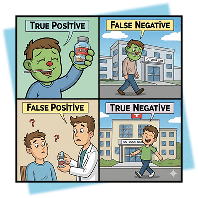
| True Positives (TP) | ✅ Your model correctly predicted the positive class. | Your model predicted a patient had a disease, and they actually did. |
| True Negatives (TN) | ✅ Your model correctly predicted the negative class. | Your model predicted a patient did not have a disease, and they actually didn’t. |
| False Positives (FP) | ❌ Your model incorrectly predicted the positive class (Type I error). | Your model predicted a patient had a disease, but they actually didn’t. |
| False Negatives (FN) | ❌Your model incorrectly predicted the negative class (Type II error). | Your model predicted a patient did not have a disease, but they actually did. |
1. Special Case – Multiclass Confusion Matrix:
A multiclass confusion matrix is a table that helps you visualize the performance of a classification model across more than two classes. The rows represent the actual labels, while the columns represent the predicted labels, similar to a binary class confusion matrix.

- True Positives (TP): The model correctly predicts class 0 as class 0. This value is found in the main diagonal, specifically in Cell1.
- True Negatives (TN): The model correctly predicts non-class 0 classes (class 1 and class 2). This is calculated by adding up the cells that represent correct predictions for other classes: Cell5 + Cell6 + Cell8 + Cell9.
- False Positives (FP): The model incorrectly predicts non-class 0 classes (class 1 and class 2) as class 0. This is computed by adding the off-diagonal cells in the class 0 column of the confusion matrix: Cell4 + Cell7.
- False Negatives (FN): The model incorrectly predicts class 0 as non-class 0 classes (class 1 or class 2). This is found by adding the off-diagonal cells in the class 0 row of the confusion matrix: Cell2 + Cell3.
Now, as the number of classes grows, you need to apply the same procedure to evaluate the TP, TN, FP, and FN. Once you have the values for these, you will be able to calculate any derived metrics.
2. Derived Metrics:
While the matrix itself gives you a visual breakdown, we can use the four values True Positives (TP), True Negatives (TN), False Positives (FP), and False Negatives (FN) to calculate more specific and meaningful metrics. These metrics provide a more nuanced understanding of a model’s performance than a simple count of correct predictions.
- Accuracy:
This is the most straightforward and common metric. It tells you the percentage of all predictions the model got right.
While easy to understand, accuracy can be misleading, especially with imbalanced datasets. For example, if you have a model that detects a rare disease that affects only 1% of the population, a model that simply predicts “no disease” for everyone would achieve 99% accuracy but would be completely useless in a real-world scenario.

- Precision:
The metric focuses on the quality of the positive predictions, minimizing false alarms. A high precision score signifies that your model rarely makes erroneous positive predictions.
It answers the question: “Of all the positive predictions my model made, how many were actually correct?”. This is critical in applications where a false positive is costly, such as in a spam filter where you don’t want to accidentally flag important emails.

- Recall:
The metric focuses on the model’s ability to find all the positive cases. A high recall score means your model rarely misses a positive case.
It answers the question: “Of all the actual positive cases, how many did my model correctly identify?”. This is crucial in applications where a false negative is a major risk, such as in a medical diagnosis model for a serious disease.

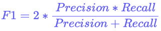
- F1 Score:
The F1 Score is a single metric that balances both Precision and Recall. It is the harmonic mean of the two, making it a great choice when you need to strike a balance between minimizing false positives and false negatives, especially with imbalanced datasets.
Let’s consider a scenario, where out of 100,000 transactions, only 100 might be fraudulent. A naive model that predicts “legitimate” for every transaction would achieve a deceptive accuracy of 99.9% (99,900 correct legitimate predictions / 100,000 total), but it would be completely useless as it misses all the fraudulent cases.
In this scenario, we don’t just want high precision (not flagging legitimate transactions) or high recall (catching all fraudulent transactions)—we need a balance. A model that only optimizes for recall might flag too many legitimate transactions as fraud, causing a poor user experience. Conversely, a model that only optimizes for precision might miss too many fraudulent transactions, leading to significant financial losses.
3. Visualizing and Interpreting the Matrix
Libraries like Scikit-learn make it incredibly easy to generate a confusion matrix. The most common way to display it is as a heatmap, which makes the values visually intuitive and easy to interpret.
import numpy as np
import matplotlib.pyplot as plt
import seaborn as sns
from sklearn.metrics import confusion_matrix
from sklearn.model_selection import train_test_split
from sklearn.ensemble import RandomForestClassifier
from sklearn.datasets import load_breast_cancer

# 1. Load a real-world, balanced dataset from scikit-learn
# The breast cancer dataset is ideal for binary classification tasks.
data = load_breast_cancer()
X = data.data
y = data.target
class_names = data.target_names # ['malignant', 'benign']

# The classes are: 0 = 'malignant', 1 = 'benign'.
# Let's check the class balance:
unique, counts = np.unique(y, return_counts=True)
print("Class distribution:")
for name, count in zip(class_names, counts):
   print(f"  {name}: {count} samples")

# 2. Split the data into training and testing sets
X_train, X_test, y_train, y_test = train_test_split(X, y, test_size=0.3, random_state=42)

# 3. Train a machine learning model (Random Forest)
model = RandomForestClassifier(random_state=42)
model.fit(X_train, y_train)

# 4. Make predictions on the test data
y_pred = model.predict(X_test)

# 5. Generate the confusion matrix
# The confusion_matrix function compares the true labels (y_test) with the predicted labels (y_pred).
cm = confusion_matrix(y_test, y_pred)

# 6. Visualize the confusion matrix as a heatmap
plt.figure(figsize=(8, 6))
sns.heatmap(cm, annot=True, fmt='d', cmap='Blues',
           xticklabels=class_names, yticklabels=class_names)

plt.title('Confusion Matrix for Breast Cancer Prediction')
plt.ylabel('Actual Label')
plt.xlabel('Predicted Label')
plt.show()

print("\nConfusion Matrix:")
print(cm)

# 7. Print derived metrics (for a more complete example)
from sklearn.metrics import accuracy_score, precision_score, recall_score, f1_score

accuracy = accuracy_score(y_test, y_pred)
precision = precision_score(y_test, y_pred, pos_label=0) # Specify positive label for precision
recall = recall_score(y_test, y_pred, pos_label=0)       # and recall since 'malignant' is 0
f1 = f1_score(y_test, y_pred, pos_label=0)

print(f"\nAccuracy: {accuracy:.4f}")
print(f"Precision (Malignant): {precision:.4f}")
print(f"Recall (Malignant): {recall:.4f}")
print(f"F1 Score (Malignant): {f1:.4f}")


print(f"\nAccuracy: {accuracy:.4f}")
print(f"Precision: {precision:.4f}")
print(f"Recall: {recall:.4f}")
print(f"F1 Score: {f1:.4f}")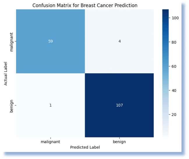
The darker or more prominent squares on the main diagonal (from top-left to bottom-right) indicate correct predictions (TP and TN), while the lighter squares off the diagonal represent errors (FP and FN). By looking at which off-diagonal squares are larger, you can instantly see where your model is struggling.
Here, the model performed very well, achieving an overall Accuracy of 97%. It was highly effective at correctly identifying both malignant and benign cases.
- True Positives (Correct Malignant): The model correctly identified 59 cases as malignant.
- True Negatives (Correct Benign): The model correctly identified 107 cases as benign.
- False Positives (Incorrect Malignant): The model incorrectly identified 1 benign case as malignant. This is also a Type I error.
- False Negatives (Incorrect Benign): The model incorrectly identified 4 malignant cases as benign. This is a Type II error.
The low number of false negatives is especially important in a medical context, as it means the model is unlikely to miss a positive cancer diagnosis.
When to use it?
The Confusion Matrix and its derived metrics are essential for evaluating classification tasks. It becomes particularly powerful and necessary when you are dealing with imbalanced datasets, where one class has significantly more samples than the other.
For example, in a rare disease detection model, a “naive” model that simply predicts “no disease” for every patient could achieve 99% accuracy if the disease is extremely rare (e.g., 1 in 100 people). In this case, a high accuracy score is misleading.
The confusion matrix would immediately reveal a high number of False Negatives (FN), showing the model is failing to detect any of the actual positive cases. Precision and Recall would provide a much more honest picture of the model’s performance.
⚠️ Common Mistakes
1. Misinterpreting the Matrix:
A common mistake is not understanding what each quadrant represents. Remember, columns are the predicted values, and rows are the actual values.
2. Wrong Metric Selection:
Don’t rely solely on accuracy. You must choose your primary metric based on the problem’s goal.
- If you need to minimize False Positives (e.g., a spam filter), prioritize Precision.
- If you need to minimize False Negatives (e.g., a medical diagnosis), prioritize Recall.
- If you want to maintain the balance between the two, prioritize the F1 score.
3. Ignoring the Context:
The “best” score depends on your specific use case. A model with 90% accuracy might be terrible for self-driving cars but perfectly acceptable for a movie recommendation system.
Continue your Journey
The Confusion Matrix is an indispensable tool in a data scientist’s arsenal. While metrics like accuracy provide a quick summary, the matrix itself gives you a rich, nuanced view of your model’s performance. By looking beyond a single number and analyzing the true positives, false positives, true negatives, and false negatives, you can gain deeper insights and select the most appropriate metrics for your specific problem. Always use the Confusion Matrix as your first step in evaluating a classification model and use its derived metrics to tell the full story of your model’s strengths and weaknesses.
To further enhance your skills and master these concepts, explore Udacity’s School of AI. This school offers a range of programs designed to give you the technical skills needed for a career in AI. For a robust foundation, consider the Introduction to Machine Learning course. If you’re ready for advanced, career-focused learning, the AWS Machine Learning Engineer Nanodegree program is an excellent choice. Start your journey to data-driven success with Udacity today!