Gone are the days where you can work as a data professional without mastery of Python. Chief among Python’s data analysis ecosystem is the pandas library, which provides efficient and intuitive methods for exploring and manipulating data. In this pandas tutorial, we’ll go over some of the most common pandas operations.
About Pandas
Pandas is among the most popular Python libraries. Its name is a portmanteau combining the phrase “panel data,” another term for multidimensional datasets. Wes McKinney, the man behind pandas, designed it to automate repetitive data preprocessing tasks. Today, pandas is more than just a data manipulation library; it allows Python programmers to efficiently perform analyses and create visualizations from their data.
This pandas tutorial provides an introduction to some of the most common data manipulation tasks without bogging you down with complex documentation and technical jargon.
Pandas Fundamentals
To use pandas, we conventionally import it as follows:

We stick to this convention to avoid errors that would arise from calling pandas methods that have the same names as Python’s built-in functions. By importing pandas as pd, we prefix pandas method calls with pd as well, to thus differentiate between two function calls that would otherwise be identical.
The following two sections describe the two fundamental pandas data structures: Series and DataFrames.
Python Series
Series is a one-dimensional object with a structure similar to that of an array. It’s capable of storing any data type, be it a numerical object, string, list or custom Python object.
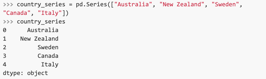
The simplest way to create a Series object is to provide an iterable of data to the pandas Series method call. In the example below, we create a Series object from a list of country names.
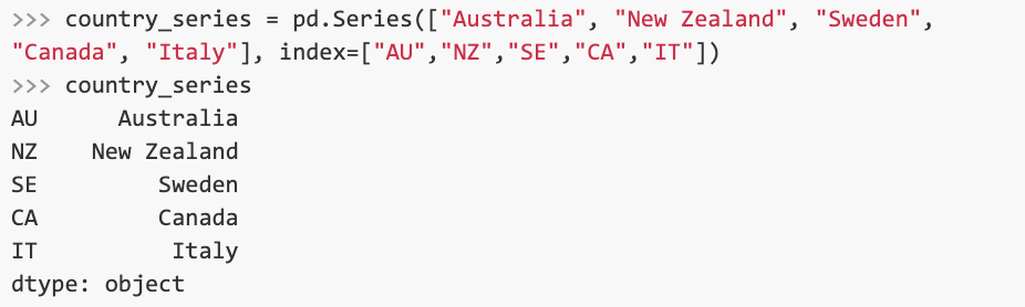
By default, pandas assigns integer indices to a Series object. However, we can specify a list of custom indices by assigning the list to the index keyword in the Series method call. In the next example, we replace the default integer indices with a list of country codes. Note that the order of elements in the two lists matters since there’s a one-to-one correspondence between the lists’ elements.
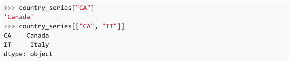
We can also specify an index or a list of indices to access a particular element or a subset of elements of a Series:
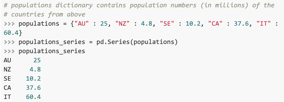
We may also construct a Series from a Python dictionary. In this case, the resulting Series object takes on the dictionary’s keys as its indices. The code snippet below illustrates this approach.
Python’s pandas library is built on top of NumPy and many of its operations also apply to pandas objects:
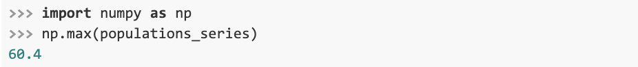
For a more comprehensive list of NumPy and pandas operations, check out our Python data analysis cheat sheet.
Python DataFrame
A DataFrame is a two-dimensional object that stores data in a tabular format, i.e. rows and columns. You could think of a pandas DataFrame as horizontally stacked Series objects with the same indices.
The most common way of creating a DataFrame from scratch is by constructing it from a dictionary. The columns of the resulting DataFrame correspond to the dictionary’s keys, whereas the rows correspond to its values. The values are typically within an array-like object.
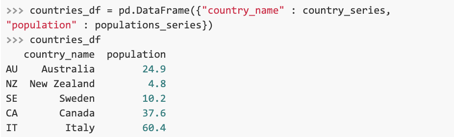
The dictionary that we used to construct our DataFrame stored values as Series objects; this works because under the hood, Series are just NumPy arrays. Note that country_series and population_series must have the same indices to be matched.
Pandas Operations
Reading and Writing Data
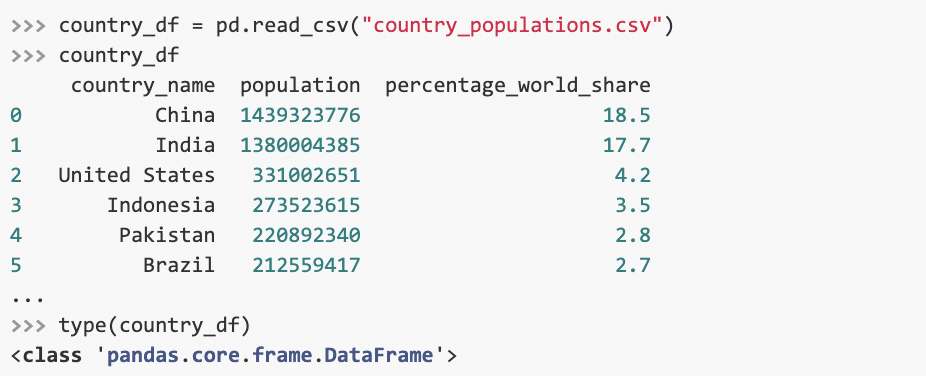
Rather than creating a DataFrame from scratch, we more often want to read data from the disk. Python and pandas provide many methods to simplify the process. For example, it takes a single method call to read a .csv file into a DataFrame:
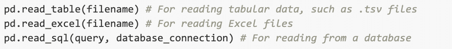
Below are some other common methods used for reading data from disk:
Equivalent methods exist for exporting data:
Data Exploration
Once we’ve imported the data into a DataFrame, we’ll want to explore it. Data exploration is a crucial step of working with data as it helps us detect issues and guide the direction of the analysis. Pandas offer many methods for quick data exploration. For example, we’re able to determine the shape of the dataset with the shape attribute:

Our dataset consists of 12 rows and 3 columns.
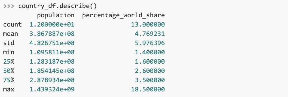
It’s often useful to display descriptive statistics about a DataFrame. Calling the describe() method on a DataFrame returns information such as the mean, standard deviation and interquartile range for all numeric columns.
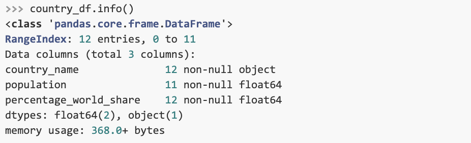
info() provides useful information about a DataFrame’s columns, data types, non-null values and memory usage.
It’s also important to visually inspect the data. head() and tail() methods display the top and the bottom rows of a DataFrame, respectively.
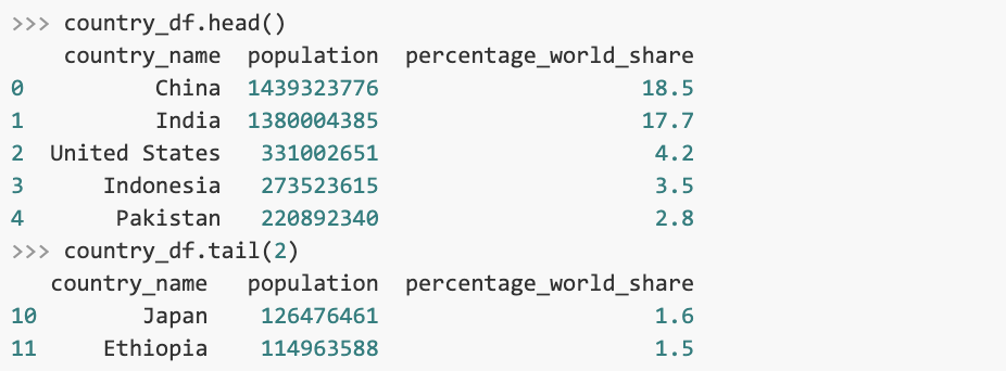
head() and tail() print five rows by default, but we can specify a different number in the method’s call.
Accessing Data in a DataFrame
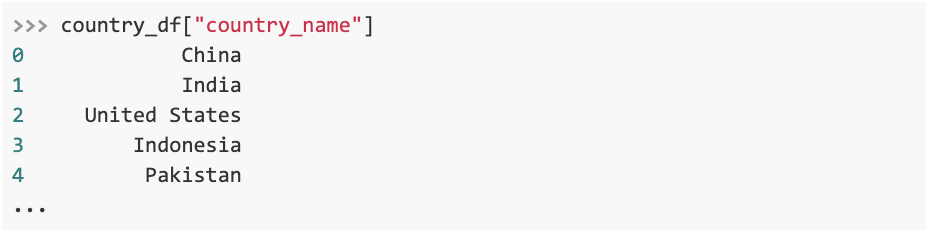
We can access a DataFrame’s column by specifying the column’s name within square brackets after the DataFrame’s name:
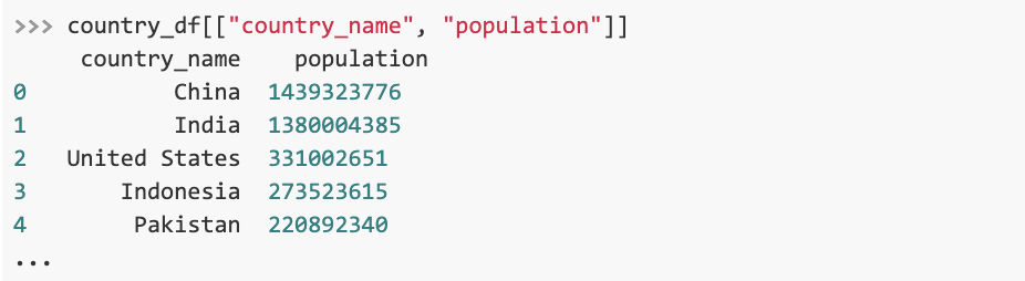
To access a subset of the DataFrame, we can index it with a list of column names:
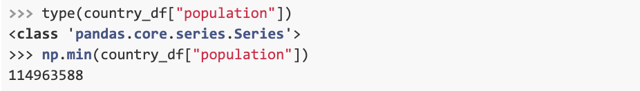
We may apply different NumPy operations to a column, since retrieving a column returns a Series object.
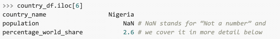
To access a DataFrame’s row, we specify the row’s index within the iloc attribute.
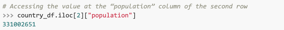
We can access a particular value by specifying both a row and a column:
Using this syntax, we can assign a new value to a DataFrame.

Inserting Data
There are many ways of adding a new column to an existing Python DataFrame. The simplest method is to access the DataFrame using the new column’s desired name — just like we’d access a dictionary, and assign it the list containing new values using the assignment operator.
In the example below, we create a list that stores True if the country’s population is larger than 300 million and False otherwise, saving this information into a new column in the DataFrame:
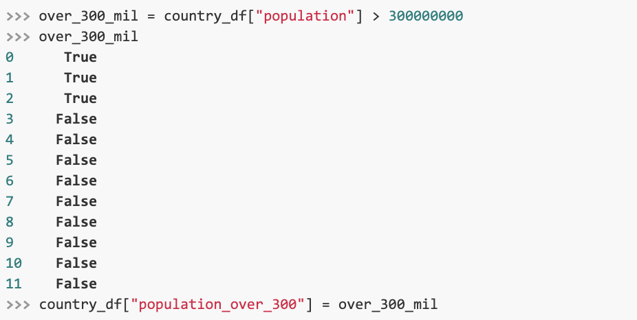
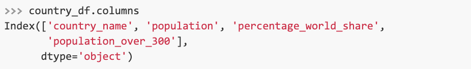
We can print the names of all columns existing in the DataFrame to ensure that the new column has been added:
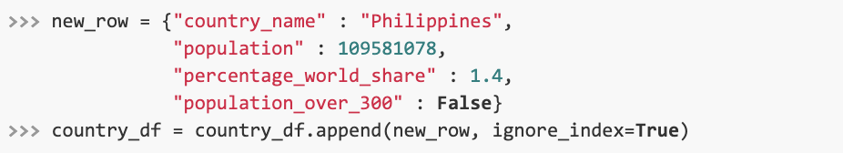
One way to insert a new row into a DataFrame is with the append() method. append() takes a dictionary with keys and values and adds the values by matching the dictionary’s keys to the DataFrame’s column names:
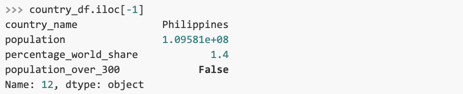
Note that the append() method is immutable, which means that instead of changing the existing DataFrame, append() returns a modified copy. Because of this, we need to assign the output back to country_df if we want to keep the changes. We can check that the row has been added by indexing the DataFrame’s last element:
Handling Missing Data
You may have noticed earlier that our Python DataFrame has the value NaN for Nigeria’s population. NaN stands for not a number and we use it to indicate missing data. Since datasets often contain missing data, pandas provide tools for handling these scenarios as painlessly as possible.
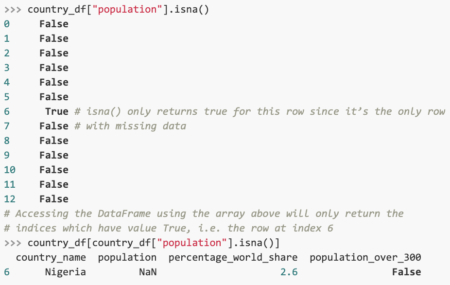
We may use the isna() method to check for missing data. isna() returns an array of boolean values, storing True for rows that have missing data and False for those that do not. Accessing a DataFrame with a boolean array returns only the DataFrame rows for which the value in the boolean array is True, i.e. the rows which have missing data. Take a look at this example:
Boolean indexing is useful because it allows us to access the missing values and change them. Here’s a relevant example of syntax:

Alternatively, we can call the dropna() method to remove the rows with missing values:
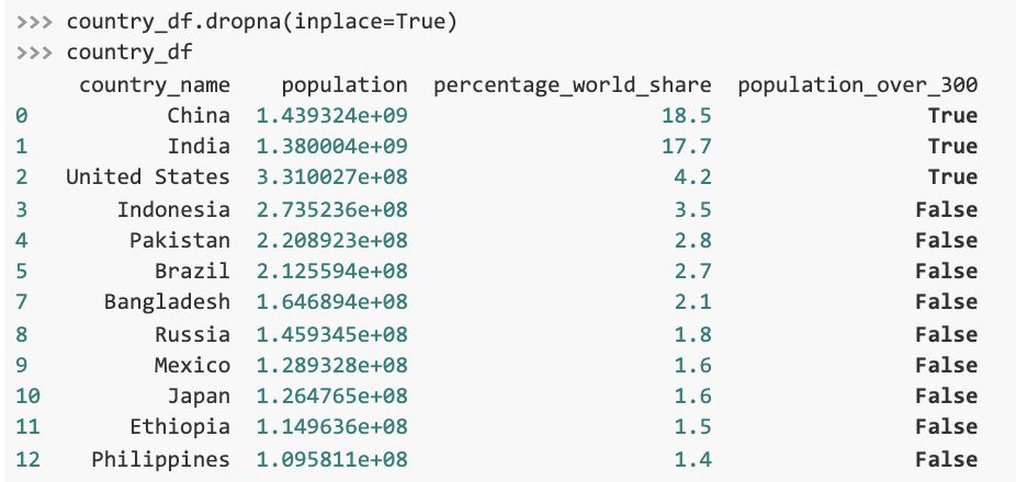
Note how the updated DataFrame does not have a seventh row. Providing inplace=True to the method call modifies the existing DataFrame. When in place is set to False, which is the default case, dropna() returns a modified copy of the DataFrame, requiring us to assign this copy to a variable.
Learn More
In this Python pandas tutorial, we covered the basics of Python’s pandas library. There’s much more you’ll learn on your road to becoming a Python programmer. Start your career in Web and App Development, Machine Learning, Data Science or AI by taking our Introduction to Programming Nanodegree.

