Last Updated on October 23, 2024
When working with data, whether for analytics or data science applications, a key step in the ETL pipeline is transforming data. Transforming data with Python is an essential skill for data engineers which includes three broad categories: manipulating the form of the data; engineering features in the data; and transforming data values.
The Python Pandas library contains a large variety of functions for manipulating data, including tools to accomplish all three types of transformations.
In this article, we will review what each of the three categories of transformation means and then see examples in Python using Pandas.
What is transforming data?
Both ETL and ELT processes have the letter “T” which stands for “transform.”During the transform step, the data engineer will perform three categories of transforms:
1. Manipulate the form of the data
This type of data transformation is an opportunity to form the data such that it is suitable for an intended purpose. Specific examples might be reordering and selecting rows; renaming and selecting columns; removing duplicate values; or handling missing values.In addition, large-scale transformations might include changing from a wide to long or long to wide format.
The goal is to have a set of data ready to be analyzed whether in a report, a statistical model, or a machine learning model.
2. Engineer features in the data
This type of data transformation generates new data values based on existing values. This is an important step for many advanced statistical and machine learning modeling exercises. Examples of feature engineering include creating new variables; replacing values; or combining or splitting values.
The goal is to generate appropriate columns of data to help an applied statistician or machine learning engineer create efficient, effective models for answering explicit questions about the data.
3. Transform data values
The last type of data transformation involves modifying data values to create a distribution appropriate for analysis. For example, a set of values in a dataset might be severely skewed or be inconsistently scaled. Examples of transforming data values include log, square root, or cube transformations; data standardizing or normalizing; or outlier removal.
The goal is to create data values suitable for various statistical and machine learning algorithms.
How to transform data with Python using Pandas.
Pandas is an important Python library for all data transformation tasks. The library contains a wide variety of tools for manipulating data. In the sections below, you will see a variety of functions that every data engineer should be comfortable using.
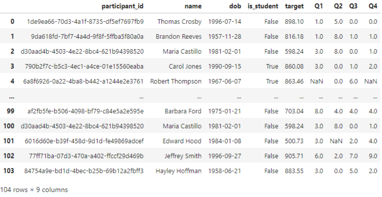
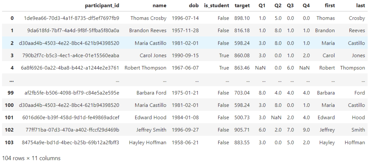
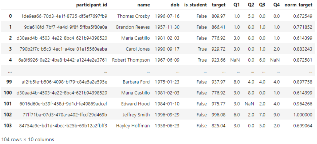
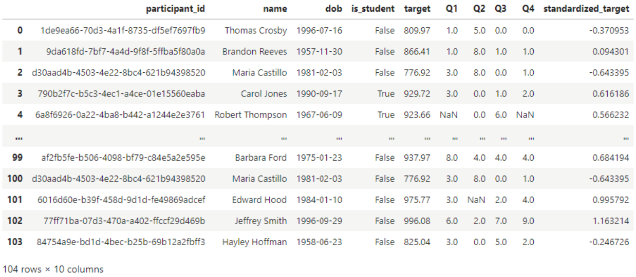
The code samples below will use this data file: student_data.csv which is a fake set of data for the purpose of this article. This code will read the data into a variable called df that will be used throughout this article. For some transforms, we will create a copy of the data frame just for convenience.
import pandas as pd
import numpy as np
import matplotlib.pyplot as plt

df = pd.read_csv("student_data.csv")
display(df)
How to manipulate the form of the data.
Changing the form of data is one of the most common use cases when transforming data using Python. Often raw data needs to be formed, reshaped, or cleaned up to be used by a data analyst or data scientist.
Sort and filter
Often the ordering of data matters, particularly when manually inspecting datasets. In addition, it can be useful to filter the dataset and only use particular rows or particular columns of data. To do this, we will use the following functions from pandas: sort_values, query, and filter.
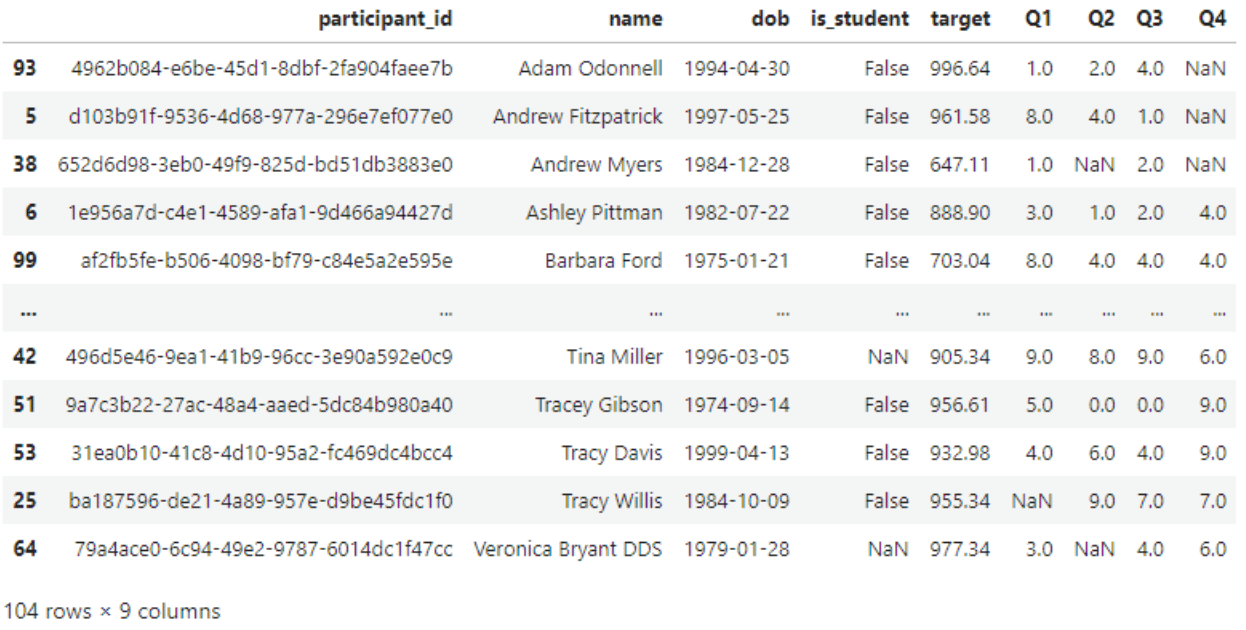
#Sort by name
sorted = df.sort_values(by=['name'])
display(sorted)
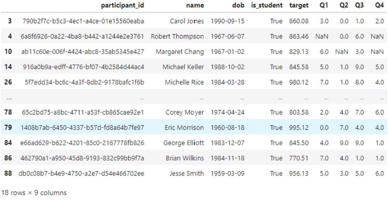
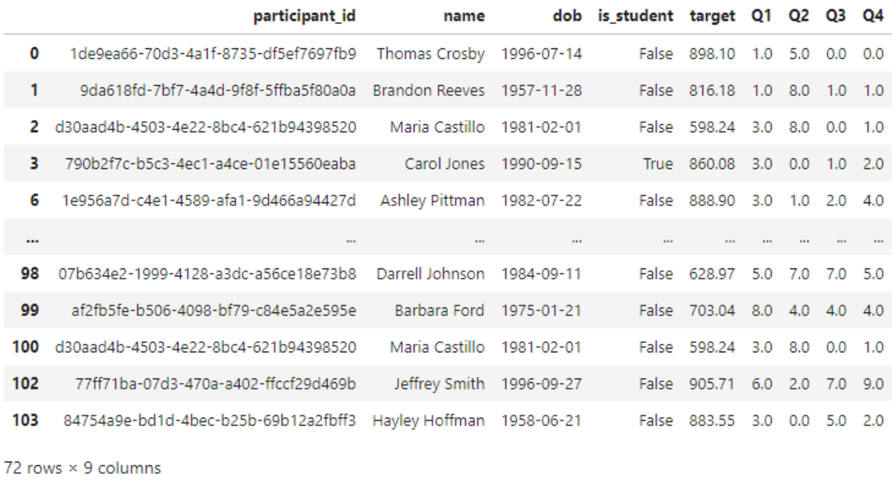
#Filter rows
just_students = df.query('is_student==True')
display(just_students)
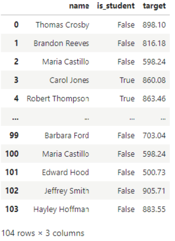
#Filter columns
no_birthday = df.filter(['name','is_student','target'])
display(no_birthday)
Removing duplicates and empty/invalid values
A common challenge with raw datasets is duplicate rows of data. Alternatively, there may be rows with only partial data. Both conditions can cause invalid conclusions from statistical and machine learning models.
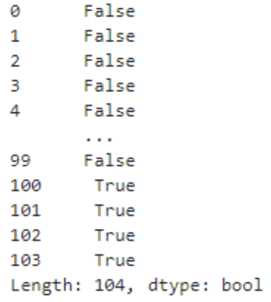
The code below demonstrates finding and removing duplicate rows using the duplicated and drop_duplicates functions. In addition, we see one technique for handling missing values called “listwise deletion” using the dropna function. First, we will use the isna function to find missing values. Note that handling missing data is a large topic and for brevity, we only cover this method but there are many other ways of handling missing values in a dataset.
#Remove duplicates
display(df.duplicated())
dups_removed = df.drop_duplicates()
display(dups_removed)
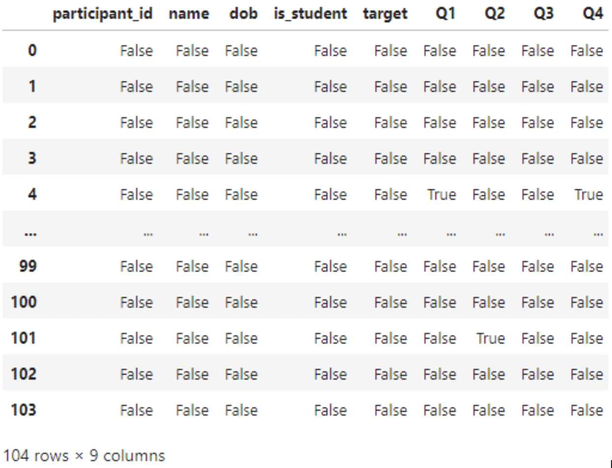
#Remove NA
display(df.isna())
listwise_deletion = df.dropna(how='any')
display(listwise_deletion)
Renaming columns
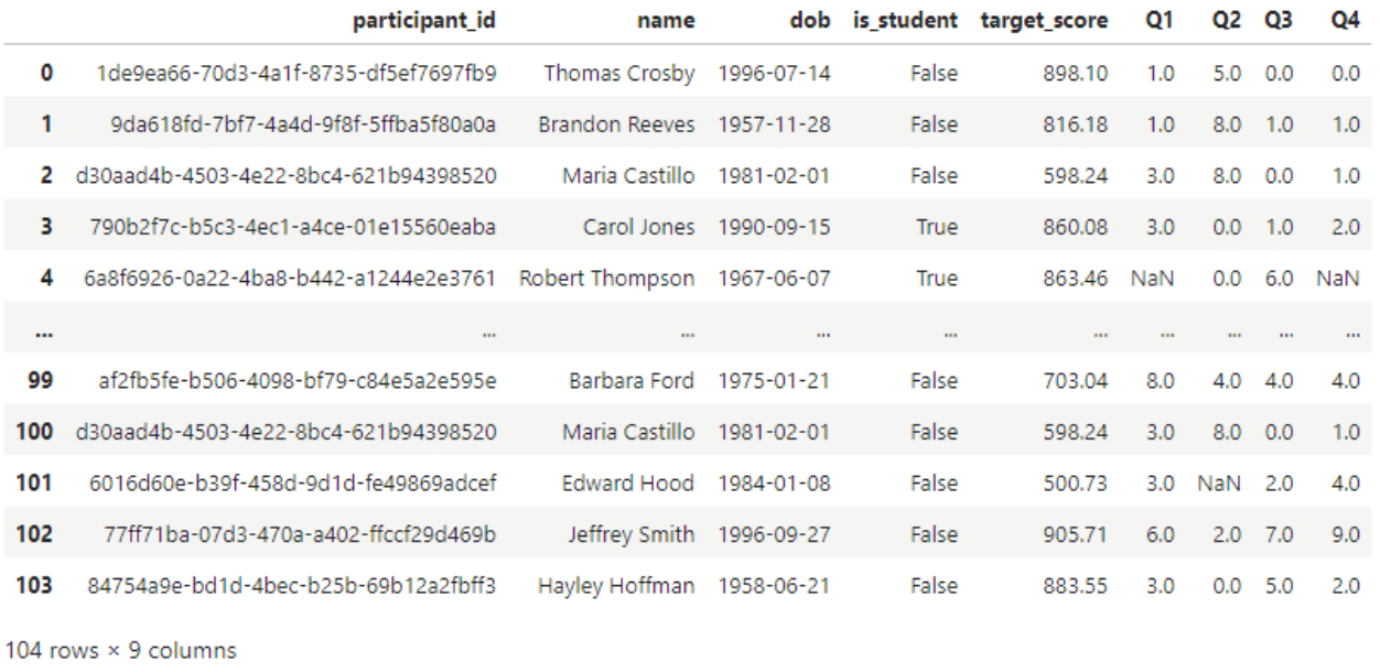
Sometimes a raw dataset will have column names that make sense to the original owner of the data but may not make sense in a broader analytic sense. The rename function allows us to change column names to something more appropriate for the data analyst or data scientist.
#Rename column
renamed = df.rename(columns={'target':'target_score'})
display(renamed)
Wide and long formats
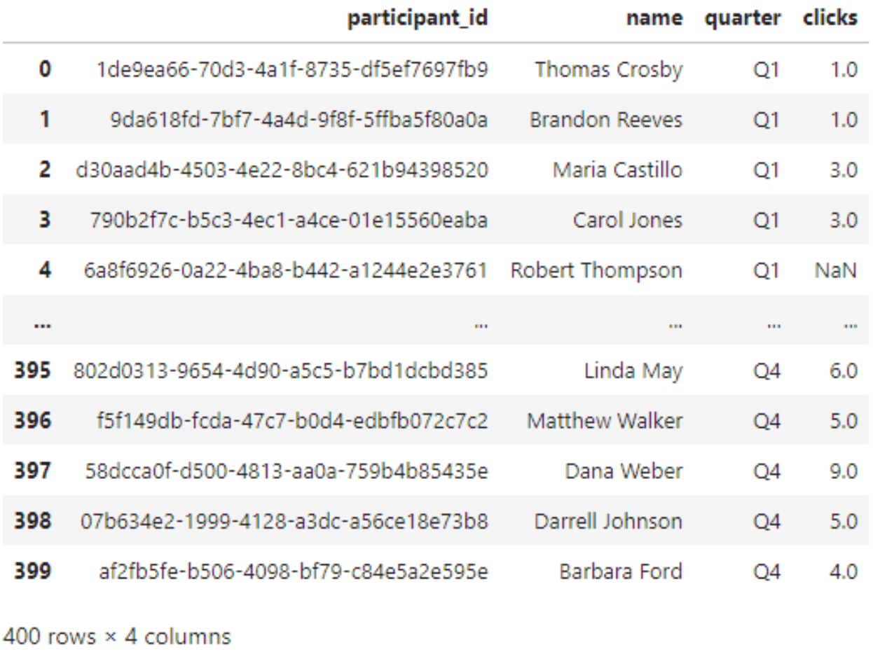
Datasets can be formatted in either wide or long formats. Wide formats are datasets that contain repeated measures or values on a single row. For example, a single record might contain values for all four quarters of a year in four separate columns. Long formats will repeat the identifying columns (id, name etc.) and then add the repeated measures on their own row such that each quarter will get its own row. Switching from wide to long we can use the melt function and from long to wide we can use the pivot function.
#Wide to long
long = pd.melt(dups_removed, id_vars=['participant_id', 'name'], value_vars=['Q1','Q2','Q3','Q4'], var_name='quarter', value_name='clicks')
display(long)
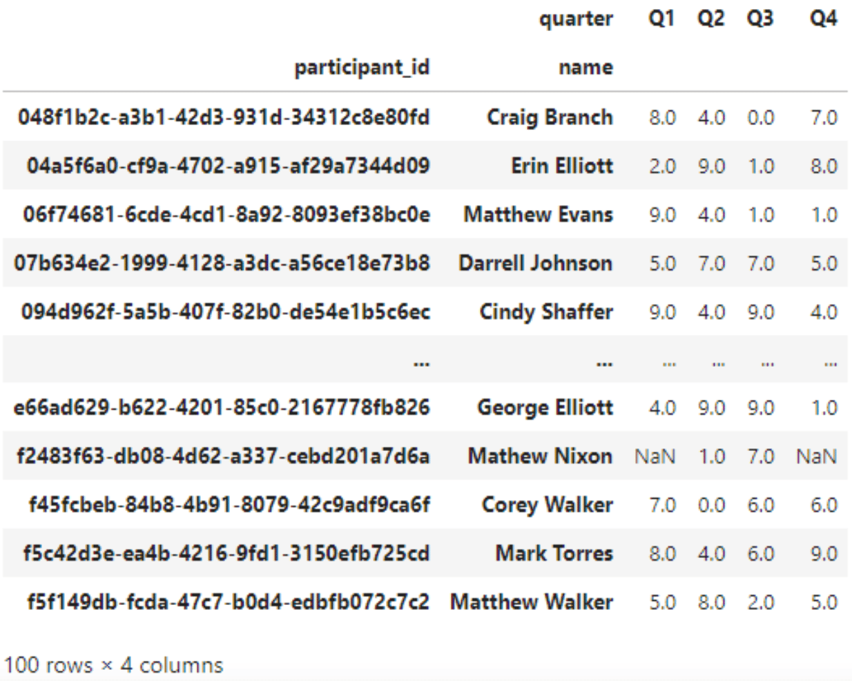
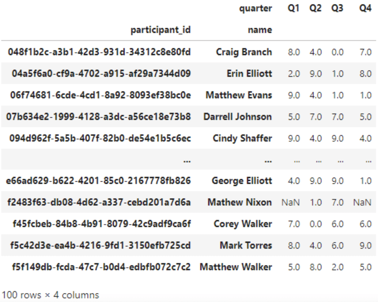
#Long to wide
wide = pd.pivot(long, index=['participant_id', 'name'], columns='quarter', values='clicks')
display(wide)
How to engineer features in the data.
Feature engineering is the process of transforming raw data into features that can be used in modeling.
For example, raw data might contain a set of continuous values but for your model, you only need to know if the value is above a certain threshold. You can engineer a feature called “exceeds_threshold” that contains a 1 or 0 depending on the condition.
The code samples below will continue using the same dataset we used in the previous section.
New variables
Another common example of creating a new variable is when a dataset contains birthdates. A more useful feature might be “age” rather than using the raw birthdate. The code below first creates a function to calculate age and then creates a new column to contain this data.
#New Variable
from dateutil.relativedelta import *
from datetime import *

def get_age(dob):
    now = datetime.now()
    age = relativedelta(now, dob).years
    return age

df['age'] = pd.to_datetime(df['dob']).apply(get_age)

display(df)
Replace values
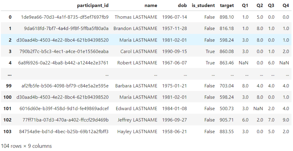
Sometimes values in a dataset need to be replaced with something more (or less) meaningful. In the example below, we are obfuscating the last name of the individual by using a regular expression to replace everything after the space with ‘ LASTNAME’.
#Replacing values
obfuscated = df.copy()
obfuscated['name'] = obfuscated['name'].replace(to_replace = '\s(.*)', value = ' LASTNAME', regex=True)

display(obfuscated)
Splitting and combining
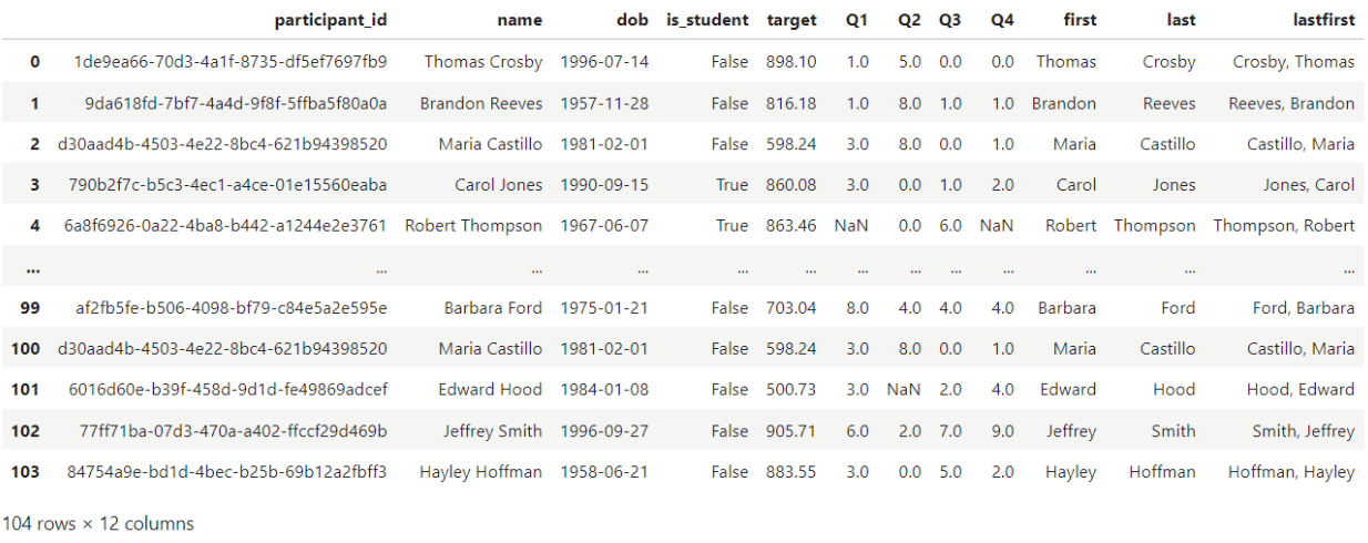
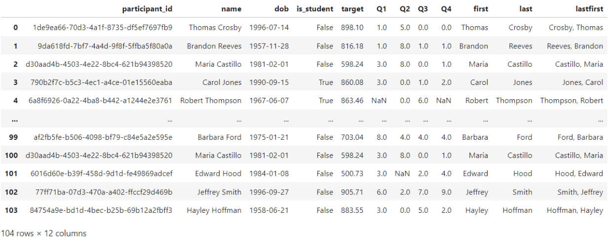
Often when working with text columns, data needs to be split and/or combined in various ways. The code below demonstrates how the name column can be split into first and last names. The next code block shows how to recombine the first and last names using the ‘last, first’ convention.
#Splitting
splitnames = df.copy()
split = splitnames['name'].str.split(' ', expand = True)
splitnames['first'] = split[0]
splitnames['last'] = split[1]
display(splitnames)
#Combining
splitnames['lastfirst'] = splitnames['last'] + ', ' + splitnames['first']
display(splitnames)
How to transform data values.
Often applied statisticians and machine learning engineers need the numeric values in data transformed to better support the assumptions of selected models. In addition, many models need data that is scaled appropriately for analysis.
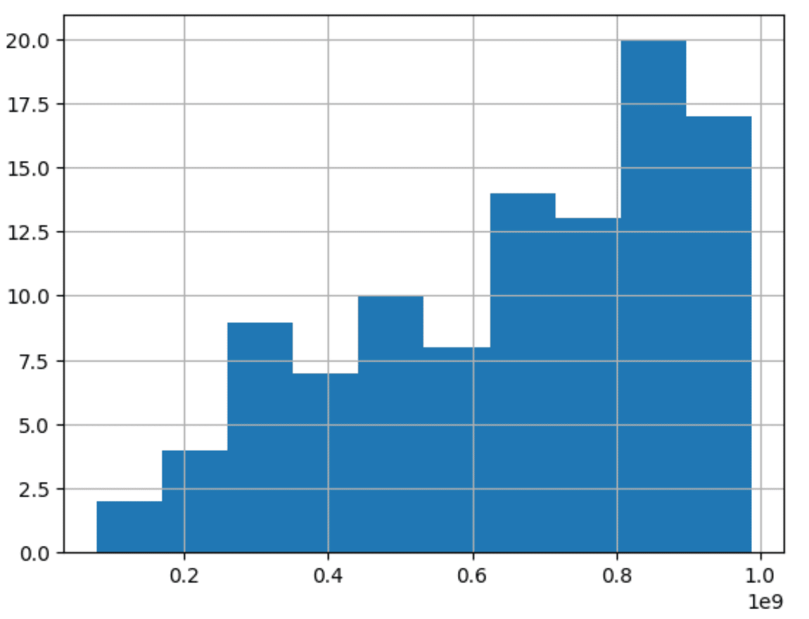
From the dataset we have been using, let’s look at the distribution of the target column.
#Data Value transforms
df['target'].hist()
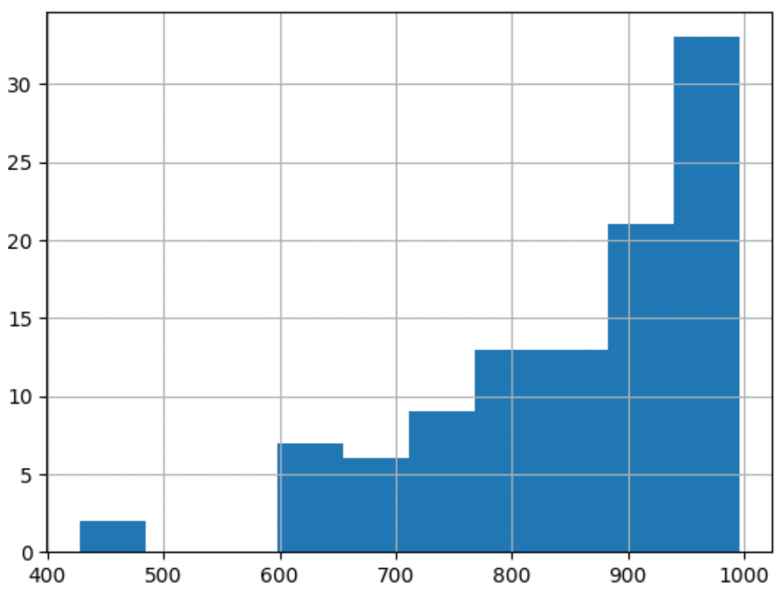
We can see this data does not conform to a normal distribution which is a common assumption for many models. In the sections below, we will look at some common transforms to see if we can transform this dataset into a more appropriate distribution.
Distribution transforms
The code below shows several different distribution transforms and the resulting shape of the new distribution.
The code below shows a log transform of the above data. Typically, we would use a log transform for right-skewed data rather than left-skewed data and we see the effect is the opposite of what we would like as it increases the skewness.
#Log transform
transforms = df.copy()
transforms['log'] = transforms['target'].transform(np.log10)
transforms['log'].hist()
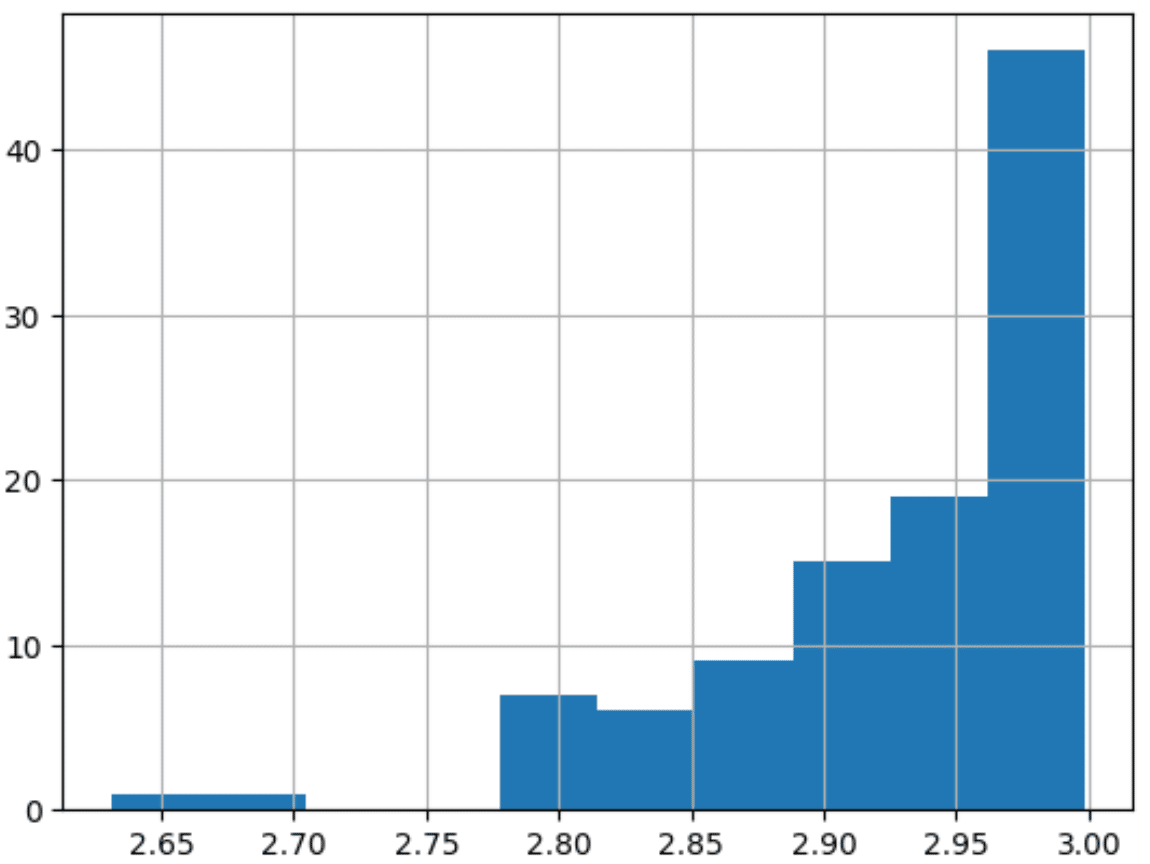
In contrast, the code below uses a cube transform which results in less skew to the resulting data. This may or may not be acceptable depending on the model being used so a data engineer would need to work with the data scientist to find the best solution. Usually, some combination of log, roots, or power transforms can be used to reshape a distribution.
#Cube transform
transforms = df.copy()
transforms['cube'] = transforms['target'].transform(lambda x: np.power(x, 3))
transforms['cube'].hist()
Scaling transforms.
When working with data columns that have varying units or scales, there are two primary methods of scaling data so the columns can reasonably be compared.
Normalization of data transforms each value to a value between 0 and 1.
Standardization of data transforms each value such that the distribution has a mean of 0 and a standard deviation of 1.
Both forms of scaling have special built functions in Python in scikitlearn to do this; however, the code below shows how to do these transforms using just numpy.
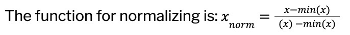
#Normalizing
scaling = df.copy()
min_target = np.min(scaling['target'])
max_target = np.max(scaling['target'])
scaling['norm_target'] = (scaling['target'] - min_target) / (max_target - min_target)
display(scaling)

#Standardizing
scaling = df.copy()
mean_target = np.mean(scaling['target'])
sd_target = np.std(scaling['target'])
scaling['standardized_target'] = (scaling['target'] - mean_target) / (sd_target)

display(scaling)
Learn to code with Udacity.
Transforming data with Python is a critical skill for any data engineer in a modern data science environment. In this article, we explained what it means to transform data, including three different categories of data transformation, and then we explored examples of each of these types of data transformation.
Want to really take your data engineering skills to the next level? The Programming for Data Science with Python Nanodegree program is your next step. We’ll teach you how to work in the field of data science using the fundamental data programming tools: Python, SQL, command line, and git.