Robots use a surprisingly simple but powerful algorithm to find out where they are on a map, a problem called localization by engineers. The algorithm known as particle filtering looks amazingly cool. In this first article, we attempt to explain the intuition behind particle filters. In part 2 we will elucidate the mathematics needed to build your own particle filters.
The Problem
Every robot that can move around, whether it is a vacuum cleaning robot like a Roomba or a self-driving car like Carla, has a lifelong problem to contend with. The problem is to find out its whereabouts on a map that every robot carries with itself. But why is finding the whereabouts so challenging? A robot can just ‘look’ at its surroundings and recall which area on the map looks like the current surroundings, not very different from how we humans find where we are in a city or inside the office when woken up from a post-lunch slumber.
The challenge is the utmost precision with which robots have to localize themselves, very unlike humans. If a Roomba thinks it is in front of a door, while it actually is slightly behind a wall, a few centimeters away from where it thinks it is, it may never be able to maneuver its way out from one room to another. A self-driving car, operating under a similar misconception, may scrape another car, veer off the road or climb a curb. The reason this does not happen is because robots are able to beat humans at one of their own games.
Humans try to address the imprecision in their beliefs by filling in missing clues using logic and reasoning but they do end up tripping sometimes. However humans move around rather slowly and have enough time to recover from a bad assumption. So, while we may miss a step on a staircase and stumble, in most cases, we do not tumble down the staircase into the abyss.
For the sake of everyone’s safety robots pack much more precision into their beliefs so that they do not have to trip and recover. How do robots synchronize their beliefs with reality so precisely? Let us find out, starting with something called priors.
Prior Beliefs aka Priors
Like us, a robot always starts with a rough first estimate of its position called the prior. How the prior is found depends on the type of the robot. In the rest of the article, we assume that the robot in question is a self-driving car or more generally an autonomous vehicle.
For autonomous vehicles, the first estimate comes from a GPS. A GPS receiver on the vehicle receives periodic pings from a constellation of satellites flying some 20,000 km above the Earth’s surface. The time difference between two consecutive pings from the same satellite is used to calculate the distance of the vehicle from the satellite which in turn is used to estimate the vehicle’s position on the surface of the Earth.
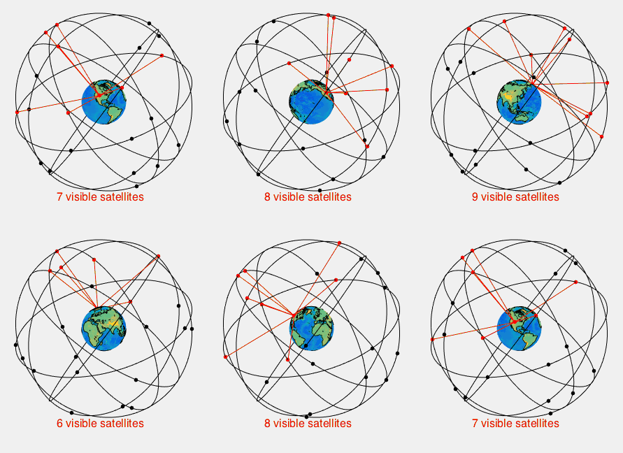
By calculating the distance from multiple satellites in a constellation, a receiver is able to narrow down its position on the planet to a few meters. However, a few meters is not good enough for a vehicle. This likely circular region around the location reported by the GPS, where the vehicle could actually be, also called a GPS spot, is the prior.
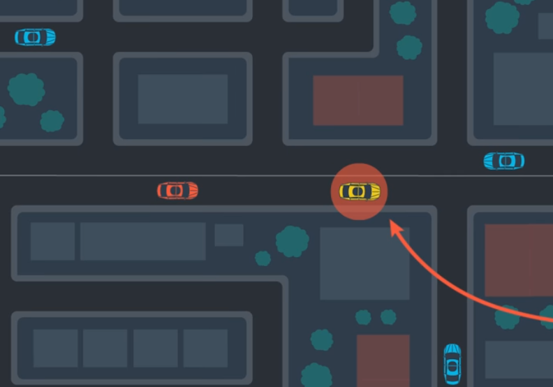
The GPS also tells the vehicle its ‘heading’, the direction which the vehicle is facing, but even the heading has some imprecision just like the location of the vehicle. To improve its beliefs about the location and heading, an autonomous vehicle uses a technique called particle filtering. We must now bring in some unnecessary analogy to drive home the point how particle filtering works.
The Intuition behind Particle Filtering
The Intuition behind Particle Filtering
To understand how particle filtering works, consider yourself in a hotel room. You wake up in the middle of the night and, to your dismay, it is pitch dark and you cannot even see yourself. You do remember crashing belly down in the bed the previous night, not caring which way your head was. You grope in the darkness and hit a water bottle, a chair and what seems like a lamp. All of these ‘small accidents’ give you clues about where you are on the bed, which side you are facing and how far you are from the edge of the bed. This iterative update of beliefs about location and orientation, using the evidence collected from your interaction with the surroundings, is the key to particle filtering.
It turns out that robots do something similar, albeit it does not involve crashing into objects to locate or orient oneself. An autonomous vehicle, for example, uses a lidar or a radar to sense the objects in its surrounding. The vehicle is able to measure its distance from these objects: trees, buildings, humans, other vehicles and so on and paint a picture of the surroundings. Using high-precision measurements, as evidence, the vehicle is able to improve its localization within the GPS spot. As the vehicle moves, so does the GPS spot and the vehicle has to repeat the process of sensing, gathering evidence and improving upon the new prior. To understand why this process is called particle filtering, let us start with the first step, which involves dividing the space inside the GPS spot into a fine grid.
Spawning Particles
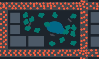
The first step in particle filtering is to divide or discretize the GPS spot into a fine grid. Shown below is a typical grid with points laid over grid positions where the car be physically present. Although the picture below shows a rectangular grid for the sake of simplicity, an actual grid is circular so that it can cover the entire GPS spot. Because the vehicle already has a map on board, it may rule out some of the areas inside a GPS spot where it is physically impossible for the car to be present, for example, what looks like, a park in the picture below.
Every feasible position on the grid is called a particle and it represents a likely position of the car inside the GPS spot. In more technical term each particle is a prior belief or simply a prior about the location and orientation of the vehicle. To represent different orientations or headings at the same location inside the GPS spot, one has to stack many such layers of particles, one for every possible orientation into a three-dimensional cube or cylinder.
To summarize, particles are more fine-grained priors, derived from a single, coarse prior provided by a GPS. WIth the priors set in place, the next step is to improve the belief or evaluate the priors against reality by sensing the environment.
Sensing the Environment
A vehicle senses its environments using a lidar or radar, both of which involve bouncing some form of energy off the surroundings. A lidar shoots light pulses in all directions and collects reflected light pulses while a radar shoots microwave pulses in all directions and collects return pings. Both have their pros and cons but in either case, what the vehicle sees is a sparse cloud of information.
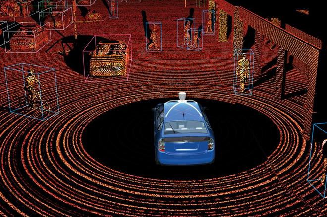
The vehicle needs to ‘connect the dots’ in the cloud and recognize objects. The picture above shows a typical lidar point cloud. As humans, we can see the outlines of vehicles and pedestrians in the point cloud but to an autonomous vehicle it is just a collection of points, that needs to be processed, to find out which points are part of which objects. This is, in itself, an interesting problem, however, in our discussion of particle filtering, we assume that objects in a point cloud have already been clustered and the clusters are categorized into different object types, and as a result, the vehicle knows which objects it is looking at and how distant those objects are. Next, we will see how the distance to these objects is used to update the beliefs.
Finding Improved, Posterior Beliefs aka Posteriors
To summarize the picture so far, a vehicle starts with a prior, a single GPS spot, which is subdivided into finer regions, each representing a likely position of the vehicle on the map, within the spot, generating multiple priors. The vehicle also has its distance to the nearby objects as well as a map with the positions of some of these objects. For the sake of simplicity, let us assume that the vehicle only keeps track of its distance from large, static objects, like buildings. The map also has the actual location of such objects, known as landmarks.
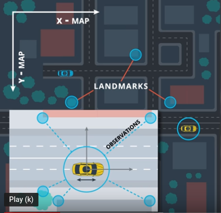
The evaluation of each prior or particle is done by assuming that the particle represents the true position and orientation of the car and then finding the distances from the particle to nearby landmarks on the map. This is very easy because both the particle’s (assumed) position on the map and the landmarks’ positions on the map are known.
To illustrate this with an example, say, the algorithm picks a particle that represents some coordinate (89.234, 77.055) and orientation 5 degrees East of North. Then it calculates the distance of nearby landmarks on the map, assuming that these are the true coordinate and heading values. Let us say that there are 3 landmarks around the particle’s location on the map and the calculated distances to these landmarks are 50.7m, 30.3m and 110.1m. If the actual distance measured by the vehicle’s lidar or radar to the same landmarks are 51.2m, 28.9m and 107.7m, the particle happens to be in the vicinity of the true (unknown) position of the vehicle. On the other hand, if the measured distances are far off from the calculated distances, for example, 32.9m, 44.5m, and 78.8m, the particle happens to be far removed from the true (unknown) position or orientation of the car.
As we saw, if the computed distances are consistent with the measured distances, the particle is highly likely to be close to the true location of the car. On the other hand, if the calculated and measured distances look very different, the particle is unlikely to be the true location. Particles with high likelihoods are retained while those with small likelihoods are discarded. So at the end of the evaluation, there are fewer particles or priors left but these priors are more reliable. These are the posteriors.
Iterative Improvement aka Filtering
As the vehicle moves, onboard sensors are able to somewhat precisely report the relative changes in its location and orientation. These changes are used to update the posteriors yielding new priors. These new priors are more reliable than the original priors but slightly less reliable than the posteriors calculated before the vehicle moved, due to the imprecision added by movement. Another round of evaluation and purging follows for these new priors and consequently, even fewer of the priors are left after the second iteration but each of the priors now is even more reliable. After just a few iterations of the evaluate-purge-update cycle, or filtering, the number of particles becomes smaller and the remaining particles have converged close to the true position of the vehicle. True to our promise, we leave you with a cool animation of a robot trying to localize itself using particle filters.
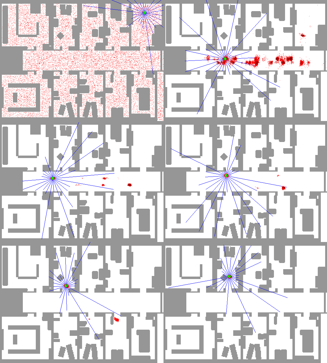
Notice how the huge number of particles, spread all over the place, collapse to a few very tight bunches of particles after a few iterations. Also, observe how, due to the symmetry of the space, there are two such bunches that exist towards the end, until the symmetry is broken, when the robot moves out of the aisle, into a room, and senses its interiors.
Udacity offers the most cutting edge courses on robotics and self-driving cars. To get an overview of how self-driving cars work, head over to this free course. If you have minimal programming experience and want to get your feet wet, we recommend our Introduction to Self-driving Cars Nanodegree. If you already have some programming experience in Python and C++ and you feel comfortable with probability and calculus, take a deep dive with the Self-Driving Car Engineer Nanodegree. If you are more interested in the walking and talking kind types of robots, the Robotics Software Engineer Nanodegree is the course for you.


